We are over a month ahead of the last partial solar eclipse on Saturday, March 29, 2025. It wasn’t a big eclipse in most European countries. Because of the largest magnitude of 0.9376, this eclipse was classified as a deep partial. Considering the Gamma factor 1.0405, the totality was visible about 210 km above the ground. Technically speaking, if, for instance, the ISS was passing roughly above that location, the observers could enjoy the view of the totality or even see a thin solar crescent on the opposite side. Staying on the ground, the observer could see the rising Devil’s horns with the obscuration of 93,1%. This text includes a report on partial solar eclipse observation from various places and explains different phenomena and the observation methods.

This is the last partial eclipse at Saros 149 before July 24, 2818. The following will be a non-central total eclipse, a rare event observable west of Kamchatka in Russia. Additionally, this is the last deep partial solar eclipse with a gamma value smaller than 1.05 before January 26, 2047. The previous deep partial solar eclipses could be observed on October 14, 2004, and November 13, 1993. Like the last one, the next eclipse will occur as early as 2051. The table below presents all partial eclipses with an absolute gamma value of less than 1.1 over the current century (Table 1).
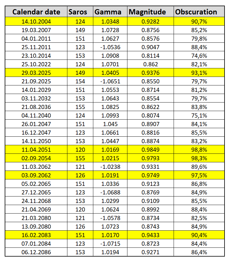
Only six partial solar eclipses with obscuration larger than 90% occur in the current century. The partial eclipse of March 29, 2025, was the fourth deepest in this century. Despite the larger gamma value, the obscuration was over 2% larger than in 2004. The reason was the position of the Moon, which was around 19 hours before perigee. In this scenario, we were so close to seeing another totality in this decade.
After these several words of introduction, let’s plunge into the observation results from different locations.
1. BASIC PARTIAL SOLAR ECLIPSE GEOMETRY
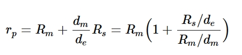
A partial solar eclipse occurs when the observer is not aligned with the lunar shadow axis, but is close enough to be located within the penumbral zone. This is the simplest definition of a partial eclipse, the most common type of eclipse. Since we consider various eclipses, such as total, hybrid, or annular, the partial phase always encompasses their paths within the penumbral zone. This time, however, the primary topic will be the geometry of the partial eclipse only. This particular type of eclipse is never central, as the umbral (or antumbral) cone misses the Earth’s surface at a closer or farther distance. Non-central solar eclipses can be annular or total, but they are rare.
The crucial value for specifying the placement of the Earth against the lunar shadow axis is the gamma value. Gamma determines how centrally the Moon’s shadow strikes the Earth. Its value is a fraction of the Earth’s equatorial radius, which is exactly 6378137 meters. The “perfect” Gamma value represents the least distance from the axis of the Moon’s shadow to the center of the Earth and could be very close to zero. The exact 0 Gamma value would require a perfect Sun-Moon-Earth alignment, which is infinitesimal. The Gamma value can be positive or negative depending on whether the shadow axis passes north or south of Earth’s center. In this case, we can’t mistake the Earth’s center with the equator line! The crucial role is played by, e.g., the Moon’s declination here. When positive, the negative gamma value can apply to the greatest eclipse at the lowest latitudes of the Northern Hemisphere and vice versa. The details of this thread will be explained in further readings. Considering the geometry of partial solar eclipses, the absolute value of gamma ranges between 1.0266174 and approximately 1.55. In contrast, a partial eclipse’s upper limiting value depends on the distance separating the Earth from the Moon.
The specificity of the March 29, 2025, partial solar eclipse focuses on a lower limiting value, which marks the extreme situation when the Moon is at perigee. Let’s consider the geometry of this eclipse in detail. First, we can compute the umbra circumstances on eclipse day.

The formula (1) below provides the most straightforward calculation of the total umbral cone length (Honey, 1918).
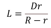
Where:
L – total length of the umbra,
D – the distance between the Sun and the Moon
R – the Sun’s radius
r – the Moon’s radius
The Moon’s mean radius can be obtained from the k2 parameter, which, for umbra calculations on the March 29, 2025, eclipse, is 0.2722810. Because the k2 parameter is measured in equatorial Earth’s radii, we can obtain the length of the mean lunar radius of 1738,1 km.
The following formula can be written accordingly in Excel:
L = (D*r)/(R-r)
For the March 29, 2025, partial solar eclipse, I took the variables obtained from the astropixels.com website, which are:
Distance of Earth from the Sun – 0.998371 au
Distance of the Moon from Earth – 359543km
Assuming that the astronomical unit (AU) value is 149597870,7km, the Sun on March 29, 2025, was 149354175,8km from Earth and 148994632,8km from the Moon. By applying these values to the formula, we receive the length of the umbral cone of 372828,8 km.
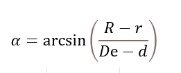 The length is the same if we consider a modern and more detailed formula (2) derived from this link. Instead of the distance between the Sun and Moon (D), the distance between the Sun and Earth (De) and Earth and Moon (d) is applied.
In Excel, the following stuff could be written as:
α = DEGREES(ARCSIN((R-r)/(De-d))
The result comes straight away in degrees, the α angle indicates the angular difference between the shadow axis and shadow edge, as per the graph on the right (Pic. 4). Once the α angle is known, we can use another formula (4) based upon the radius of the Moon to compute the total length of the umbral cone.
The Excel notation could look as follows:
L = r/(SIN(α)*PI()/180)
Finally, the total length of the umbra on March 29, 2025, obtained from these two formulae, counts exactly 372826792m.
Since the distance of the umbral cone from the Moon is the same as previously – 372827 km, we are sure that the eclipse would be total if it touched the Earth’s surface elsewhere. As mentioned above, the gamma value of this eclipse was 1.0405 and defines the distance from the Earth’s center. Regarding the distance of the shadow axis from Earth’s surface, we must realize that the Earth is flattened due to its rotation. In turn, the difference between the equatorial radius and polar radius is about 21km.
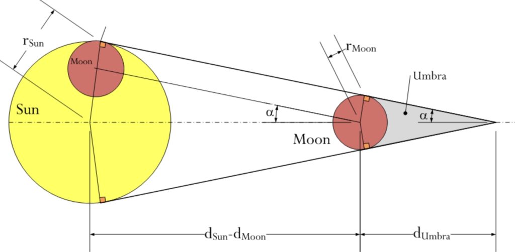
 Whereas the equatorial radius is approximately 6378 km, the polar one is only 6357 km. In practice, each latitude on Earth has its radius, which can be computed efficiently using the formulae available in this link. At first (5), the difference factor (f) between the two principal radii must be calculated. Then the difference factor (f) will be 1/298.257223563 = 0,00335286, the common Earth’s flattening factor.
 It is essential to apply the final formula (6), which can compute the length of the Earth’s radius for any latitude. Because the latitude of the greatest eclipse of March 29, 2025, was about 61 degrees north, our approach should look as follows:
=SQRT(((a^2*COS(∅*PI()/180))^2+(b^2*SIN(∅*PI()/180))^2)/((a*COS(∅*PI()/180))^2+(b*SIN(∅*PI()/180))^2))
As the Excel cells represent the following variables:
a = Equatorial radius
b = Polar radius
∅ = Latitude
At a latitude of 61,1004 degrees (or 61° 6’1.44″), the Earth’s radius is roughly 6361779m.
Last, we can consider the Gamma value and make the relevant corrections. Because the Gamma value estimation for the Earth’s equatorial radius was 1.04053, it technically means that the shadow axis was located at 6636,6 km from the Earth’s center. When defining the “height” of the shadow axis above the Earth’s surface on March 29, 2025, we must subtract the latitude 61 Earth’s radius from this value. Finally, we can confirm that the shadow axis passed approximately 275 km above the Earth’s surface. This distance can still be subject to correction, as all the geodetic features are neglected here.

Since the altitude of the umbral center is known, we need to define the rough altitude at which this eclipse would be observed as total. Earlier, we had calculated the umbra cone length as 372828,8 km. This distance is longer than between the Moon and Earth on that day. Therefore, we should consider the umbra diameter “above our heads”. To understand how it works, we can look at the graph above (Pic. 5), which shows the relationship between the umbral diameter and the Earth’s surface. Indeed, the example resembles ideal eclipse conditions, typical of near-zero Gamma values, at which the umbral shape is circular. Imagine that the same projection of umbra (s Umbra) is moved from the Earth’s surface to the vertical line at the extension of the Earth’s radius. We would still see the  circular umbra there. The main image above (Pic. 3) could hint at understanding it, assuming that the Gamma line is extended beyond the umbral cone and acts as the plane.
By applying the formula above (7), we can easily calculate the diameter of the umbra projected onto the plane above. The formula includes the subtraction of the Earth’s radius, and it’s undoubtedly correct, but only for all central eclipses, when the shadow axis hits the Earth’s surface. We don’t have a situation like this for all the non-central eclipses, especially the partial ones. In light of the definition of lunar distance, the point of greatest non-central eclipse shall be treated as the point of the Earth’s center. Therefore, the subtraction of the Earth’s radius won’t be needed at all in our case. Finally, the Excel formula will look as follows:
ru = 2*(L-d)*TAN(α*PI()/180), where:
L – total length of umbra
d – lunar distance
α – the α angle computed at formula two and explained earlier (Pic. 3).
giving a final diameter of 123,9 km. As we know, the distance of the shadow axis from the Earth’s surface at the greatest eclipse point is 275km. Now, we need to subtract the computed umbral cone’s radius from the Earth’s radius. The simple equation is: 275 – (123,9/2) = 275 km – 61,9 km = 213,1 km.
Without any geodetic assumptions, these “school homework” calculations gave us a distance of 213,1 km to the closer umbra boundary. According to NASA calculations, this distance was 208 km.
 Now it’s time for more advanced calculations, which can specify the local conditions of the greatest eclipse point. The eclipsewise.com website tells us that the eclipse magnitude was 0.938. Before we start calculating it, let’s compute the total width of the penumbra on March 29, 2025, when the greatest eclipse occurred.
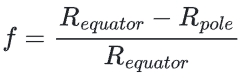
The formula on the left (8) can help us determine the radius of the penumbra by applying the following values:
Rm – The Moon’s main radius
dm – The Earth-Moon distance
de – The distance between the Sun and Earth,
Re – the Earth’s equatorial radius
Rs – the main radius of the Sun.
Concerning the traditional Excel notation based on the cells assigned, the formula above (8) would look like:
rp = Rm*(1+((Rs/de)/(Rm/dm)))
and for the March 29, 2025, eclipse, the circumstances give the penumbral radius of 3414,4 km. We don’t need to know the diameter, as the eclipse isn’t central. Moreover, we need to divide this distance between the umbral and penumbral zones, which will now be easy. Considering the umbral radius length as 61,5 km ,we have the simple substractions:
3414,4km – 61,9km = 3352,5km.
1 – 0,938 = 0,062 (by knowing the greatest magnitude of 0,938)
3352,9km * 0,062 = 207,9km
 The value of 207,9 km corresponds to the distance between Earth’s surface and the closer limit of the umbra. The same approach could be done in reverse sequence, but it’s unnecessary, as the magnitude of the greatest eclipse is already calculated. Out Of interest, the left-hand-side formula (9) is presented, which works for all non-central eclipses. However, by non-central eclipses, we can understand here also all the central eclipses right outside of their geometrical paths. Additionally, the formula can be applied for estimating the eclipse magnitude above the ground within the Earth’s atmosphere, or finaly from some satellite position. The components taken into account are as follows:
rp = penumbral radius
ru = umbral radius
Du – distance between the umbra limit and Earth’s surface (or a random point above the Earth’s surface).
Another matter of curiosity could be the outreach calculation of the greatest eclipse magnitude in the Earth’s atmosphere. As the observer would have seen the “darker sky above his head,” we shall consider the maximum altitude at which the daylight sky is completely black at zenith. This quaint thread hasn’t been discussed widely here, except for the brief explanation in this article. For the sake of simplification, we can assume that a situation occurs in the ozonosphere, at the lowest altitude of around 40km, which clearly divides the primary from secondary twilight. The atmosphere below this altitude is dense enough for the appearance of blue sky. If this is so, the estimated eclipse magnitude could be obtained e.g. from the latest formula, where we can consider the Du value shorter by these 40 km. Finally, we should get:
((3414,4 – 61,5) – (207,9-40)/(3414,4 – 61,5) = (3352,9-167,9)/3352,9 = 0,95
The greatest eclipse magnitude at an altitude of 40 km was 0,95. The last thing that comes to my mind is a calculation of the eclipse obcuration based upon its magnitude. These two things are often mistaken, as some sources don’t explain them well. Since the eclipse magnitude defines the fraction of the solar diameter hidden by the Moon, solar obscuration informs us about the percentage of the solar disk covered by the Moon. It happens very rarely that these values are the same! It’s explained under this link. Analyzing the greatest March 29, 2025 eclipse point, for the Moon-Sun ratio of about 1,03 and magnitude of 0,938, the obscuration of the solar disk was 93,1%. The hypothetical observer floating at 40km would see the deep partial eclipse with a magnitude of 0.95 and the obscuration of 94,5%. Considering the solar brightness of -23.907 Mag for the ground-based observer, at an altitude of 40 km, the solar brightness was -23,661 Mag. This means that the sun was approximately 125% brighter on the ground! Of course, we still neglect all the atmospheric impact. The scene’s brightness at the ground was 52,36 Lux and 40 km higher, only 41,74 Lux.

We are done with all the greatest eclipse computations, valid outside the ground. As we “hit” the Earth’s surface, the way of computation must change. Instead of the fundamental plane, we will look at the sphere, although all the geodetic features are still neglected for simplification. For the eclipse circumstances observed on Earth’s surface, we can use, for example, the Besselian elements. Sticking to the point of greatest eclipse, the first approach will be to specify the curves of equal magnitude (Meeus, 1989), but they must be precise to the specific time circumstances (Pic. 8). There is no total or annular eclipse this time, so it might be harder to imagine the essence of this phenomenon. The most trivial explanation of the umbral shape during the eclipse is based on the local eclipse circumstances. An ideal, almost circular-looking shape applies to the eclipses with a near-zero gamma value. Any other situations will make the umbral shape more oval. The most extreme oval shape is observed near the terminator line. Because the umbra indicates an area of magnitude of at least 1, imagine that outside of the umbra, we can theoretically mark a larger area enclosed within the specific magnitude. Eventually, we can draw the curves of equal magnitudes within the entire penumbra. The graph on the left (Pic. 7) shows the projection difference between the fundamental plane, applied outside of the Earth’s surface, and the equatorial plane, where the Moon’s shadow is observed. Any type of umbra projected on the equatorial plane far from the sphere’s center will be misshapen towards an oval. The oval-shaped umbra projection also takes place when it’s cast not perfectly onto the surface of the circular body. Unlike the fundamental plane, where any umbra is projected as a circle, or its part in the situation, when it misses the plane partially, the same umbra will have an oval shape. The same applies for penumbra sketched for equal magnitude limits, even when a larger area is considered (Pic. 8). Eventually the penumbra looks like grand outline curve on the Earth’s surface comprised of all the points at which the eclipse is beginning or ending at the given time (Gurnette, Woolley, 1961). An analog penumbra oval can be represented by the umbra, antumbra, or even the curves marking the exact duration of non-central eclipses.

The penumbra oval, specified by equal magnitude limits, changes in size and shape as the eclipse progresses (Pic. 9). It starts to appear from the terminator line, where it disappears thereafter, creating finally something like the semicircular arc. Usually, their appearance occurs along the line indicating the greatest eclipse at sunrise and ends at the line indicating the greatest eclipse at sunset, but it’s not a 100% rule. Most exceptions can be found by types V and VI of solar eclipse concerning the region of visibility (Meeus, 1997).

The appearance of the umbra or penumbra in any configuration on Earth’s surface is the clear result of the geometric position of the shadow of the Moon relative to the Earth, which is characterized by the Besselian elements. They can calculate the presence of the umbra or penumbra at the given time. In our situation, we would need to repeat all the computations done above for the location at which the “black sunrise” (or “black moonrise”) was observed. The Les Escoumins was located by the St. Lawrence River in South Quebec. The progress of a solar eclipse is shown by the movement of the umbra or penumbra across the Earth’s surface. By March 29, 2025, the solar eclipse we deal with the penumbra only, and the whole eclipse scenario can be seen in the video below.
Vid. 1 The animation of the partial solar eclipse of March 29, 2025 (In-the-sky.org)
This eclipse occurred at the lunar ascending node, so the penumbra moved slightly up. Considering the direction of Earth’s rotation, we shall see that the ascending node partial solar eclipses will always culminate at sunrise. Following the graphic eclipse progress patterns proposed by Anhert (1971), we can indicate three major moments in the image below (Pic. 10).

The image above shows the eclipse’s progress, from which we can understand one crucial thing. The Gamma value, as indicated in all the eclipses listed, for example, in the Five Millennium Catalog of Solar Eclipses (Espenak, Meeus, 2008), as well as the other data related to this value (magnitude, coordinates, solar azimuth, solar altitude, and central duration), indicates the moment of the greatest eclipse! This is the moment II in the image above (Pic. 10) and represents the smallest lunar elongation to the Sun. All the computations demonstrated above were applied to this moment – the moment of greatest eclipse elsewhere on the globe. Sometimes, like in the case of “black sunrise” captured from Les Escoumins, the additional knowledge would be necessary. The same as above, the key element will be the Gamma value, which isn’t the same as at greatest eclipse. For better understanding, I would say that the case of I and III corresponding to the beginning or the end of the eclipse elsewhere on Earth will apply to the Gamma value of about 1.55, as discussed at the beginning of this text. The correct computation of the Gamma value for the eclipse culmination at Les Escoumins can be done by this simple formula on the right (10).
This formula includes the following: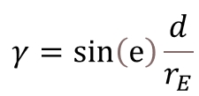
e – the elongation of the Moon (in degrees)
d – the distance between the Earth and the Moon
re – the Earth’s equatorial radius
The trickiest can be the calculation of the lunar elongation here. When you open some astro software like Stellarium and select the Moon from where the eclipse occurs, you will be informed about its elongation against the solar disk. This is not the right way to get it from there! The lunar elongation can be considered only from the subsolar point, which indicates the location directly under the Sun. This location corresponds to the Earth’s very center. The real-time information about the sub-solar and sub-lunar points is usually available on any Day and Night World Map. Below the map, the coordinates of both the sub-solar and sub-lunar points can be found. Now it’s a straightforward way to estimate the angular distance between these two bodies, and later, the Gamma value. For these calculations, I will use the most commonly available, although not precise enough, the TimeAndDate service, which gives the following coordinates:
Sub solar point – 3°34′ N, 25°11’E = 3.56667 N, 25.18333 E
Sub lunar point – 4°22′ N, 24° 27’E = 4.36667 N, 24.45 E
Now it’s straightforward to compute the angle between these two coordinates. They can be done from the formula below (11):
![]()
where the φ corresponds to latitude and λ to longitude. The Excel notation can be found right beneath.
=DEGREES(ACOS(SIN(lat1*PI()/180)*SIN(lat2*PI()/180)+(COS(lat1*PI()/180)*COS(lat2*PI()/180)*COS((lon1–lon2)*PI()/180))))
According to Stellarium 25.1, the lunar elongation at the sub-solar point was approximately 1°06′, so 1,1 in decimals. Now, let’s apply the Gamma calculation (10) formula, which is based on the lunar elongation and will give us a value of around 1.08. When understanding the sub-lunar point, the lunar parallax doesn’t exist because the Moon shines directly overhead. This formula can also be applied to point out the Moon’s elongation beyond the geometrical range of a solar eclipse, when its impact on twilight is observed. Additionally, for some curious reasons, the Gamma value can be calculated even if the eclipse isn’t observed on Earth’s surface, because in some extremely rare cases the eclipse event could be noticed from the spacecraft’s altitude, whilst from a ground perspective we have the typical New Moon phase. More explanations about it will be posted in the future.
By returning to our earlier computation, let’s skip through them carefully and list the following:
– The distance from Les Escoumins to the lunar shadow axis is 436,1km
– The distance from Les Escoumins to the umbra – 436,1 km – 61,9 = 374,2 km
– The eclipse magnitude at an altitude of 40km – 0,9
– The eclipse obscuration at an altitude of 40km – 88,1%
and finally compare them with the most excellent eclipse point in the table (Tab. 2).

Tab. 2 The crucial parameters of the partial solar eclipse of March 29, 2025 between the location of greatest eclipse and the culmination of partiality in Les Escoumins.
The difference of just about 1% in eclipse obscuration between the Les Escoumins grounds and altitude of 40km didn’t have significant impact on the sky brightness overhead.

2. THE FIRST “BLACK SUNRISE” IN HISTORY
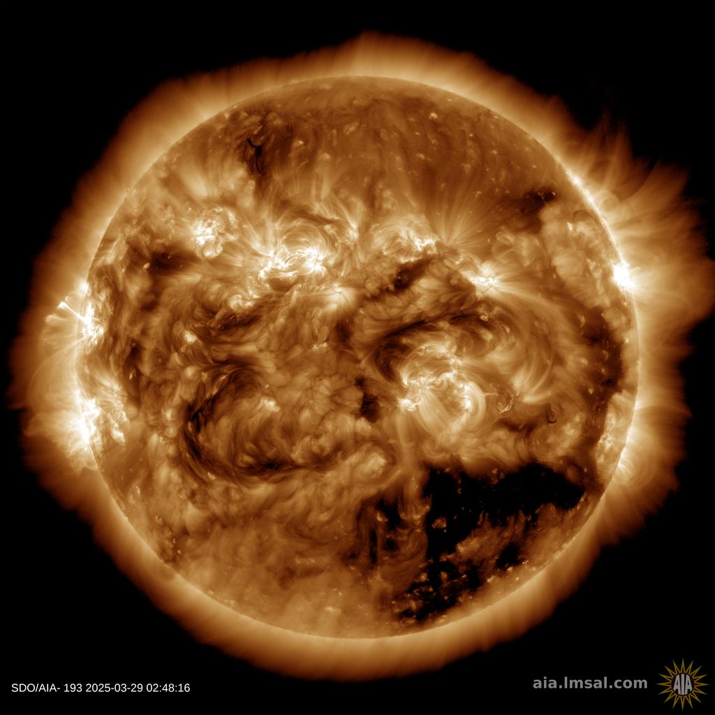
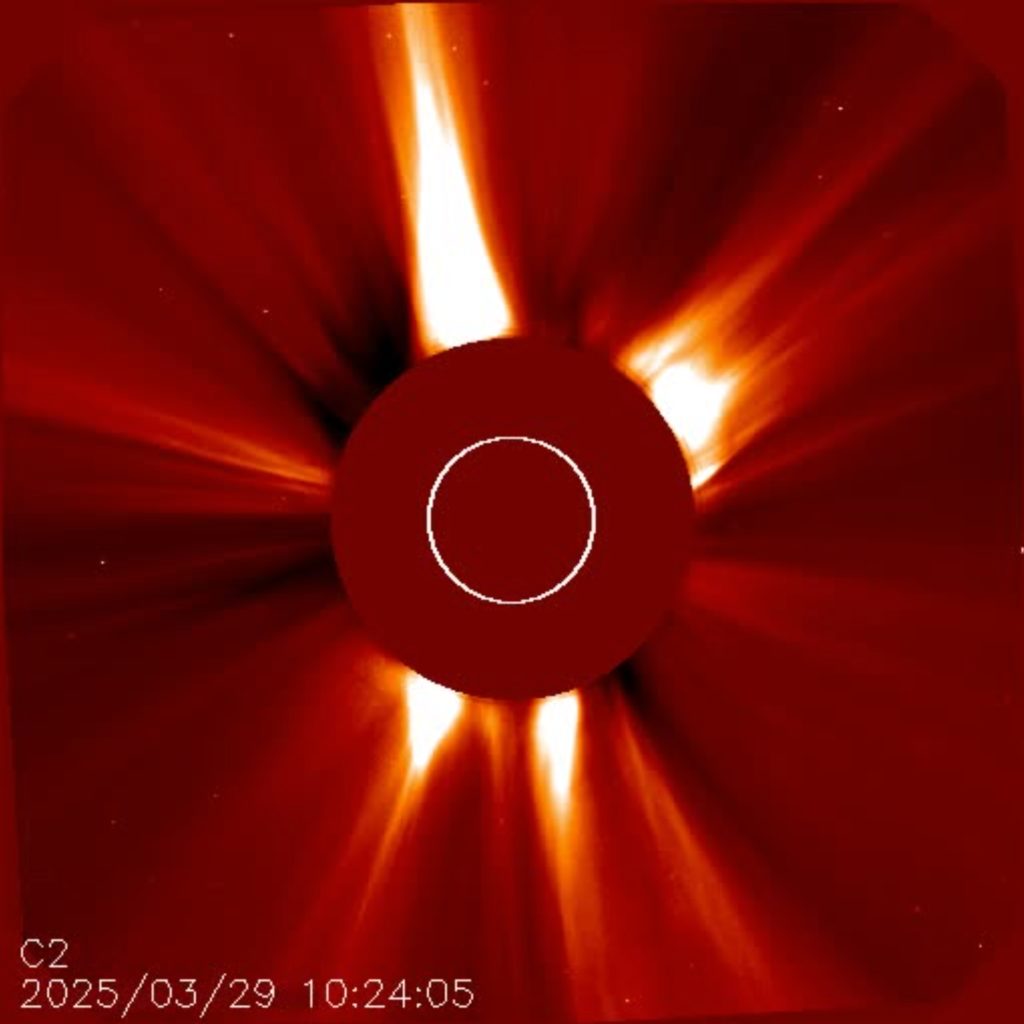
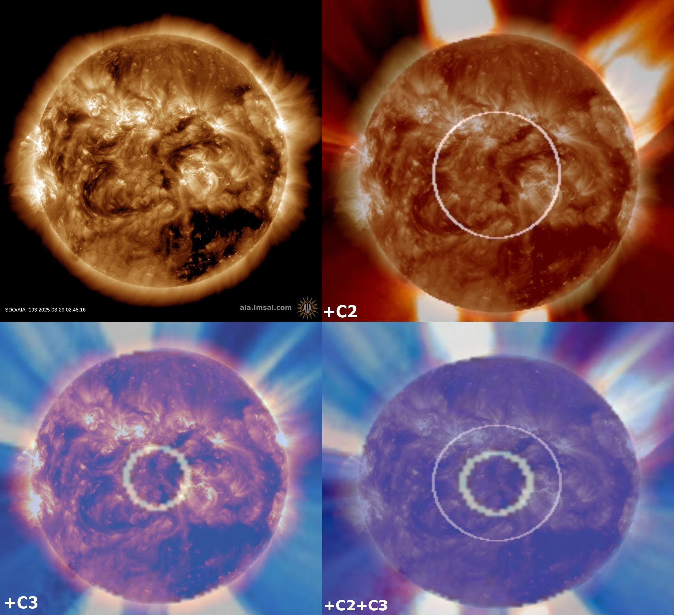
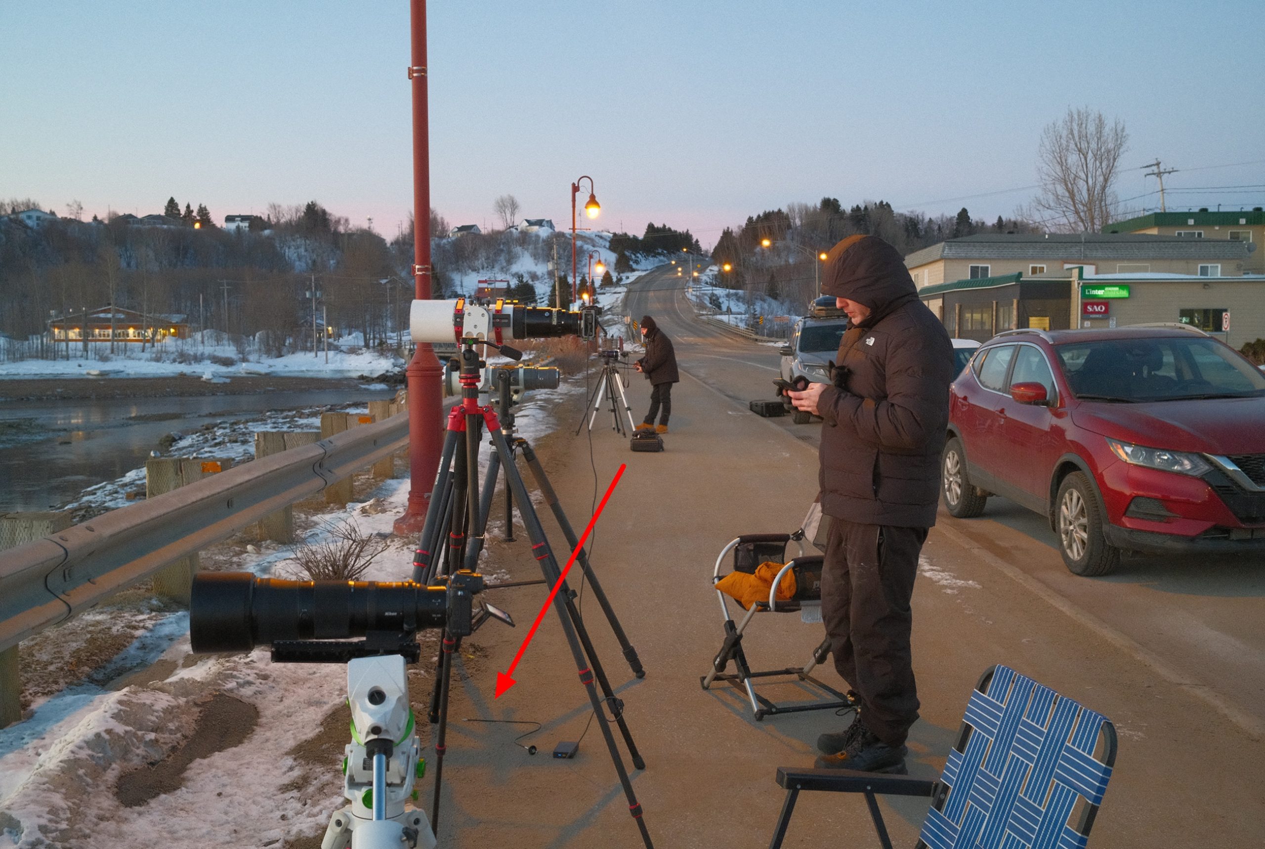
The visibility of the solar corona during the partial solar eclipse of March 29, 2025, wasn’t obvious. Probably nobody was capable of noticing it being on site. It might have gone unnoticed due to awaiting the rising devil’s horns, and people’s sight was concentrated on the illuminated clouds instead of the section of sky just above them, where the faint corona outline was visible. Indeed, I am sure it was, as the 4K videos provided by the observers prove it. One of them was Jason Kurth, who watched this unprecedented sunrise at Les Escoumins and posted it later on Facebook’s Solar Eclipse Chasers group. Despite the video quality compression made by Facebook, I noticed some “outline” roughly at the extension of the horns, which disappeared after several seconds as they rose up. Meanwhile, this video was picked up as the APOD video the next day. I could see it slightly better on YouTube. Next, by courtesy of Jason Kurth, I could analyze and process the original video, which also covered the moments before the horns went up, note bene, the most important moments as far as the optical matter is concerned. After that, I became sure that this is the solar corona outline! Additionally, I was able to spot that this outline isn’t uniform across the timing and position against the rising lunar disk. Before I demonstrate my analysis, let’s see what the solar corona looked like on March 29, 2025 (Pic. 12).
Next, I was able to detect some brighter areas based on this image and perform the detailed analysis for Jason Kurth’s video frames in 10s (Pic. 13, 14).

All the analyses based on local contrast modification and haze removal, followed by the negative RGB projections, led to official conclusions that the solar corona outline was visible that day for the obscuration of only 87%! Jason officially announced it on his Instagram profile on April 2, 3 days after the eclipse. I continued the investigation based on the coronal holes image obtained from Spaceweather.com. Because of the video length (over 4 min) including over 2m30s of analysis it was necessary to project the lunar disk movement across the Sun over this time (Pic. 15). I might be the first one, who spotted the corona outline, unless Vinod Kumar Vijayakumar did it by making single frame high quality images and the video from Lakeview Restaurtant at St. Agatha in north Maine, USA where the obscuration was only 85,9%!!! (Pic. 18, 19). However, all his images posted shortly after the eclipse report only show the picture-perfect “devil’s horns” whilst nothing indicates that the corona outline was visible to him. He used a Nikon Z6iii with a TT Artisans 500mm f/6.3 lens, so I would guess it wouldn’t be visible by the naked eye, despite its faint visibility on Facebook’s compressed image.

The visibility of the solar corona at such low obscuration is always the reason for excitement and surprise. It’s not the first observation where the view of the solar corona in similar circumstances was proven. There are other records made, i.e., by Jorg Schoppmeyer, who captured the corona view under similar obscuration conditions at least twice in eclipse history. However, these observations have one common denominator: the size of the lunar disk. Whilst the ratio of angular lunar diameter to the solar diameter on March 29, 2025, was over 1.03, in previous cases it was smaller than 1. When this ratio is smaller than 1, we deal with annular solar eclipses. It’s not a subject of consideration for now, it will be explained better later. For now, it is essential to mention that once the lunar disk is smaller than the solar one, the enclosing solar crescent shortly before the annularity reveals deeper corona structures. We don’t have a situation like this, when the lunar disk is bigger than the solar one. The deepest and brightest structures of the solar corona are hidden by the lunar disk, especially if it’s not perfectly aligned with the Sun in deep partial solar eclipse conditions. This is precisely what occurred on March 29, 2025, in Quebec. In light of these circumstances, observing the solar corona at an obscuration of barely 87% could be more difficult.
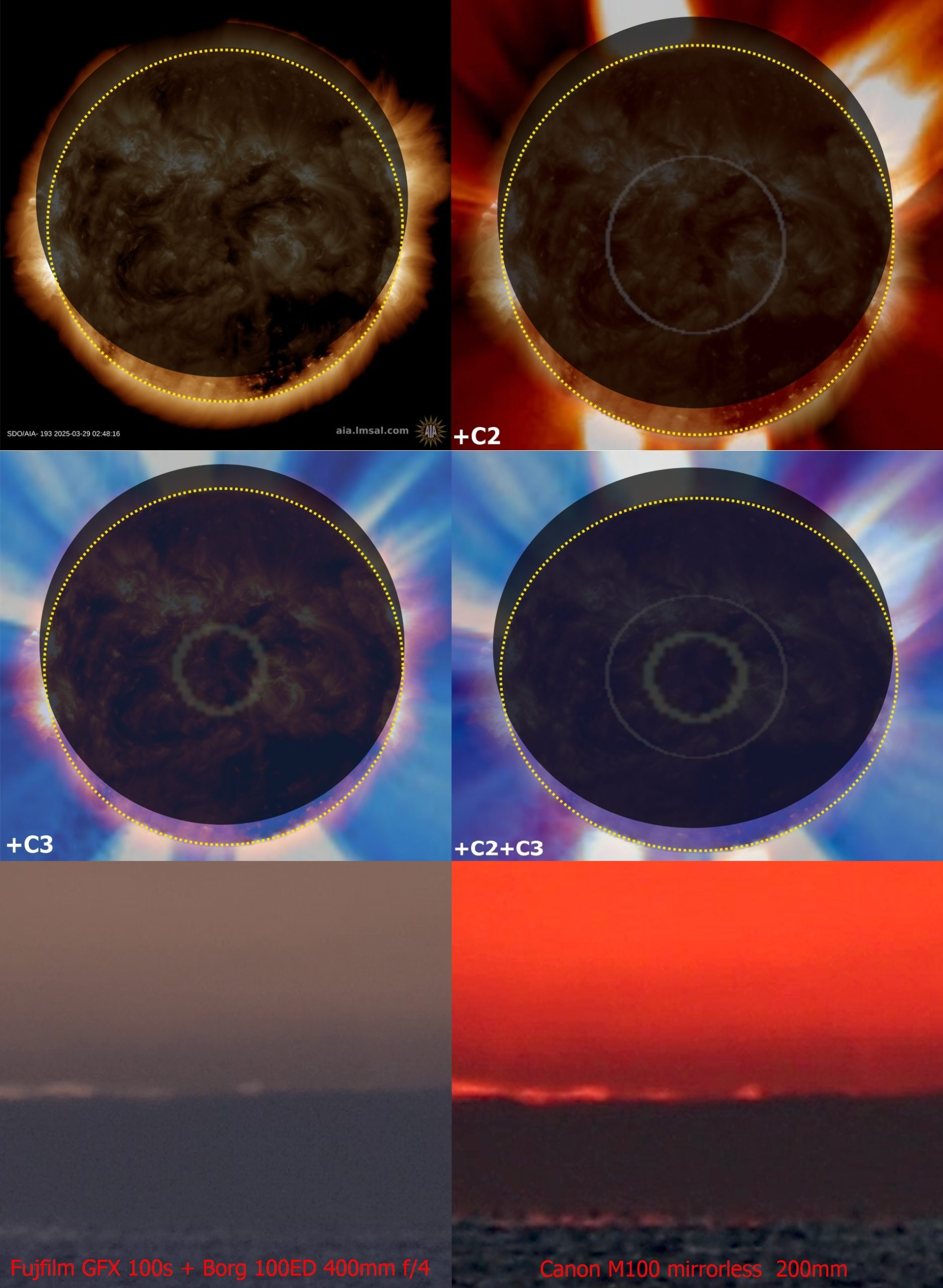
The image of solar corona holes (Pic. 12) helped me to identify some brighter features detectable by Jason Kurth’s device (Pic. 16 – 18). He used the Fujifilm GFX 100s with the Borg 100ED system 400mm f/4.


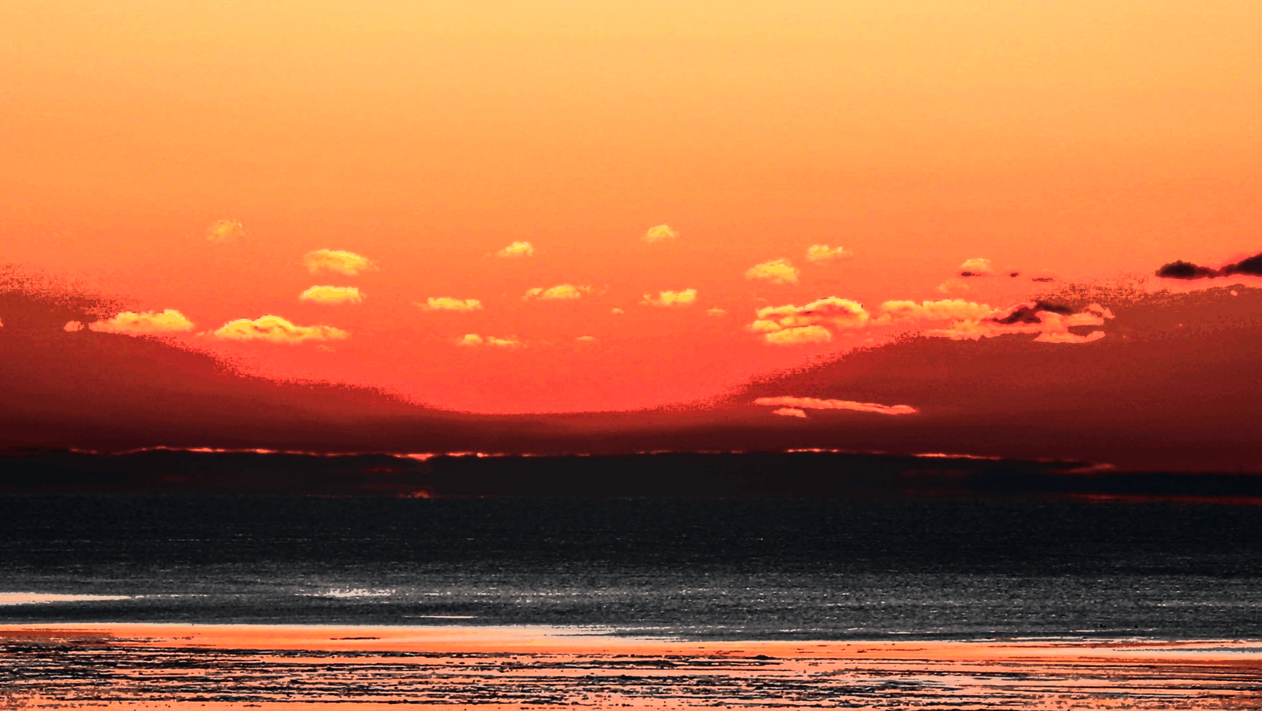
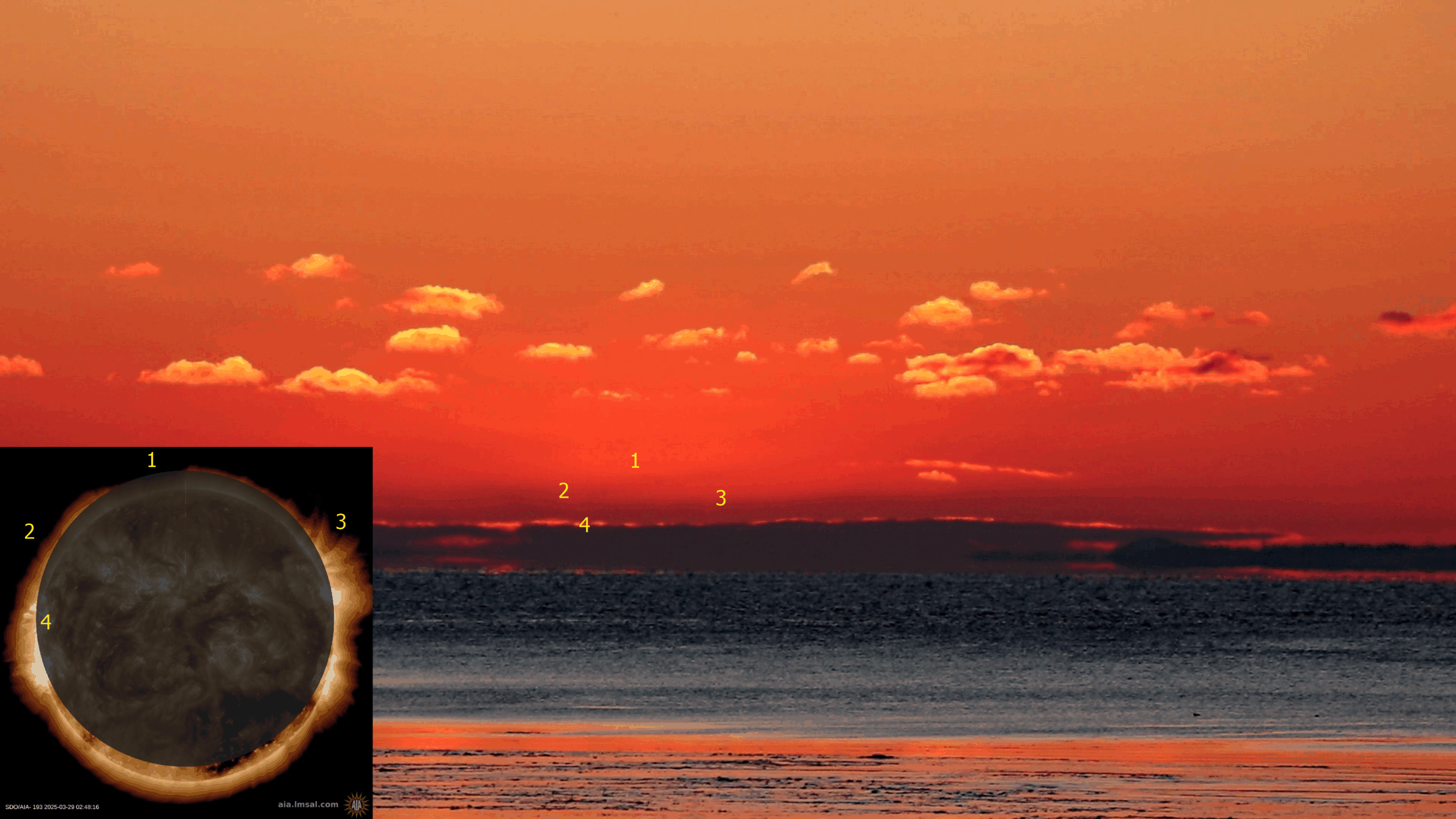
The faint solar corona was accompanied by other optical phenomena visible to the observers standing by the St. Lawrence River on the eclipse morning (Pics. 19 – 20). They are presented and explained below.
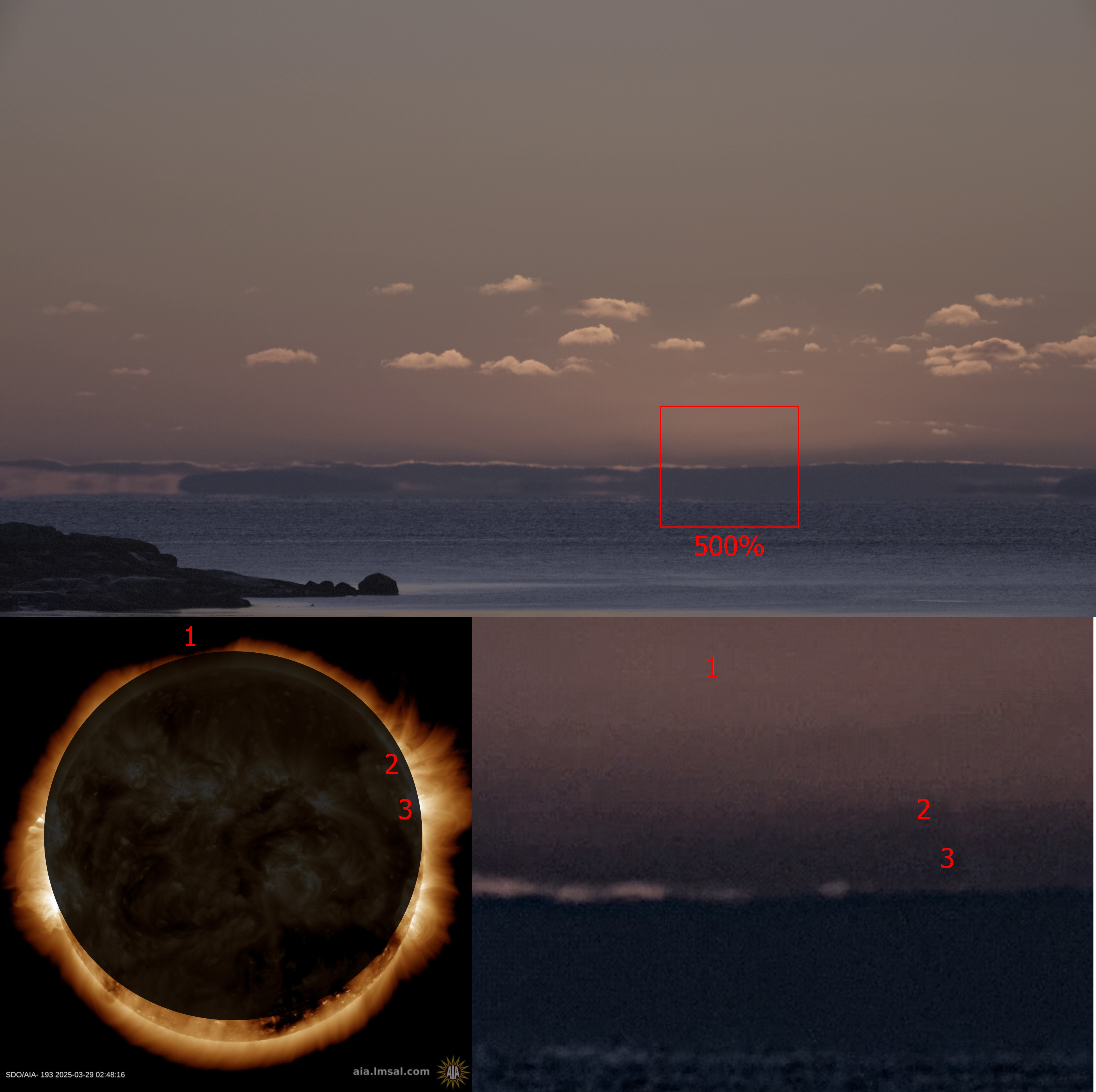
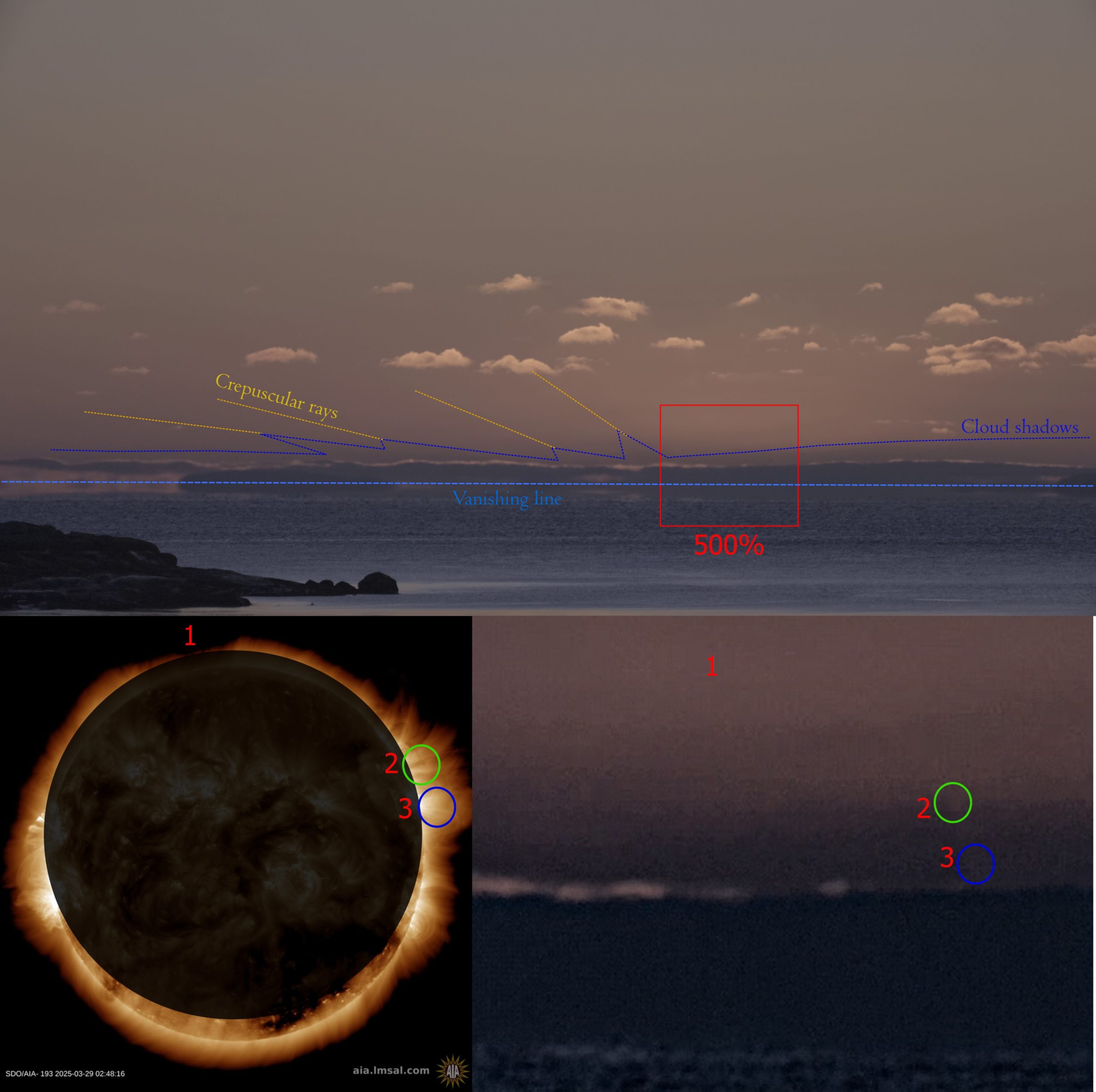
The last image (Pic. 20) indicates what optical phenomena observers were dealing with. The eclipsed sunrise occurred in strong freezing conditions. Another eclipse observer, who watched the same sunrise just 30m next to Jason Kurth, Mike Kentrianakis, reported the temperature of -13°C from his car dashboard. The Ogimet service shows almost the same temperature (Pic. 21), approximately an 18°C difference from the St. Lawrence River water temperature. It explains nicely the presence of the vanishing line, which has made the horizon invisible to the observer. Instead of it, the objects located slightly up are presented as being reflected on the water surface. In reality, their light is bent just above the water. It’s an effect of inferior mirage, which happens in the lowest part of the air being heated up by a much warmer surface underneath. This optical phenomenon was rather complex to detect by the observers focused on eclipse observations. It came up well in the videos provided, as we can see all the apparent illuminated gaps in the cloud deck and the opposite bank of the St. Lawrence River doubled just above the water surface. More information about the vanishing line phenomenon can be found in this article, which can prepare you for the 2026 total solar eclipse.
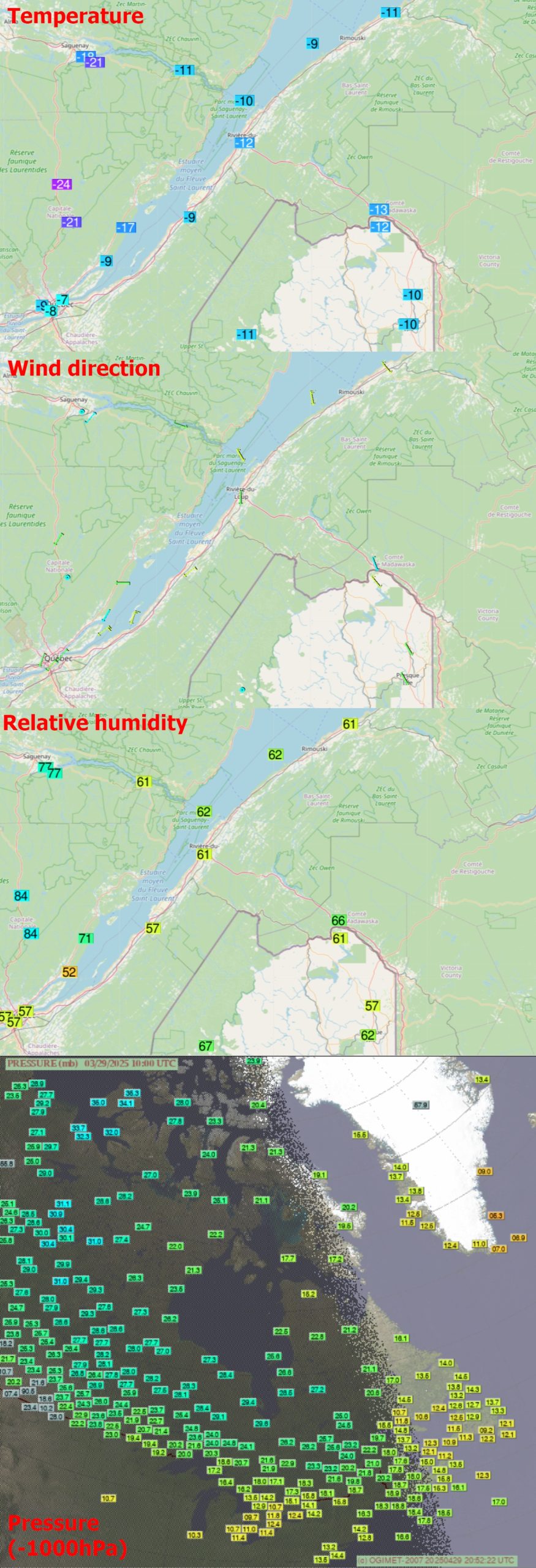
The area of Les Escumins was probably under a continental polar airmass with the strong influence of a high-pressure area located west of the St. Lawrence River and moving eastward. The pressure at 10 am UTC was about 1022 HPa. The close presence of the center of the high-pressure area resulted in slight winds with various directions shown on the map (Pic. 21). Very important is the humidity estimated locally around 43%, which increased towards the east, reaching around 58-60% right above the St. Lawrence River. It also explains the presence of green flashes accompanying this spectacular eclipsed sunset. The planetary boundary layer included a probable moderate level of haze, which, combined with the humidity level, allowed for the pronounced shadow cast by the remote cloud deck to be seen. The planetary boundary layer traps all the air pollutants, the vast majority of aerosols, and reaches usually up to 1,5 – 2km above the ground. Above this layer, the atmosphere is very clear. The layered cloud deck was probably an effect of capping inversion, which is typical for the upper limit of the planetary boundary layer. However, this inversion was near the end, as the clouds were disappearing. From the observer’s perspective, the shadow produced by this cloud deck was the most interesting, significantly reducing the forward sunlight scattering on aerosols and humidity particles within the planetary boundary layer. As an outcome, observers could see the pristine atmospheric conditions just above the planetary boundary layer within the shaded section of the sky. This thread has already been described in this article. The cloud’s shadow made a well-pronounced transition between the shaded and illuminated sections of the sky, which shows how big the difference is when the forward light scattering occurs, especially when the lowest part of the atmosphere isn’t clear enough. The layered clouds produced by capping inversion are usually uniform; however, in the case of the deep partial solar eclipse at sunrise, when instead of a full disk just two horns were initially visible, the clouds’ slight nonuniformity was expressed by the faint crepuscular rays visible to the observers left of solar azimuth. Because the shaded section of the sky allowed looking into the “clear atmosphere” above, everyone theoretically could see the faint solar corona rising along with the Moon’s disk before the devil’s horns. As the eclipsed Sun rose, this band of shaded area was reduced due to the perspective effect. It finally disappeared as the Sun’s horns became visible to the observers.
Inside the shaded section, the faint solar corona was visible. The overall brightness of the solar corona can be equal to 0.23 of the light of the full Moon (Sytinskaya, Sharonov, 1963), which corresponds to around -11 mag. In this situation, it should be easily visible even in daylight, but is ordinarily drowned out by the brightness of the Sun itself, unless we use coronographs. Even so, this task is difficult, except at the solar limb, because the solar corona, compared to the Sun, is extremely faint. Its brightness ratio compared to the Sun is as little as approximately 10-6, which is the value right outside the solar limb. By moving away by a single solar radius from the limb, the corona brightness ratio decreases to 10-9 (Golub, Pasachoff, 2010). That would correspond to the value of 0,133 Lux and 0,00013 Lux respectively, making it effectively invisible on the daylight sky, which from a ground-level perspective is brighter by 3-5 orders of magnitude (Golub, Pasachoff, 2010). Moreover, this is the average corona brightness estimation, which depends on the level of solar activity. In 2009, for example, the maximum brightness was estimated at a ratio of only 0.4 * 10-6 (Hanaoka et al. 2012). This is another matter for further writings, but we can imagine the range of changes within the brightness of solar corona (especially the K-corona), which are undeniably translated into their visibility conditions at various obscurations of deep partial solar eclipses. These events give an occasion to spot the faint corona outline by various devices or even by the naked eye. However, the minimum obscuration at which it’s possible is the live subject of investigation, and the last observation is the best example. We also need to be aware that the Earth’s atmosphere at various altitudes (even those considered for the upper limit of the planetary boundary layer) is thinner, which is expressed predominantly in a darker sky visible above our heads. Theoretically, the limit of apparent magnitude, by which the given celestial object could be visible under daylight conditions, is pushed beyond “typical” limits. In practice, it would then apply the shaded section of sky, which revealed quite good visibility of the solar corona outline. The last, however very important thing is the recent solar activity. As the Sun is around its peak of activity, it results in significant brightness in solar corona. Basically the brightness of solar corona is one of the important indices of solar activity (Sakurai, Rusin, Minarovjech, 2004). The solar cycle also determines the overall shape of the corona.
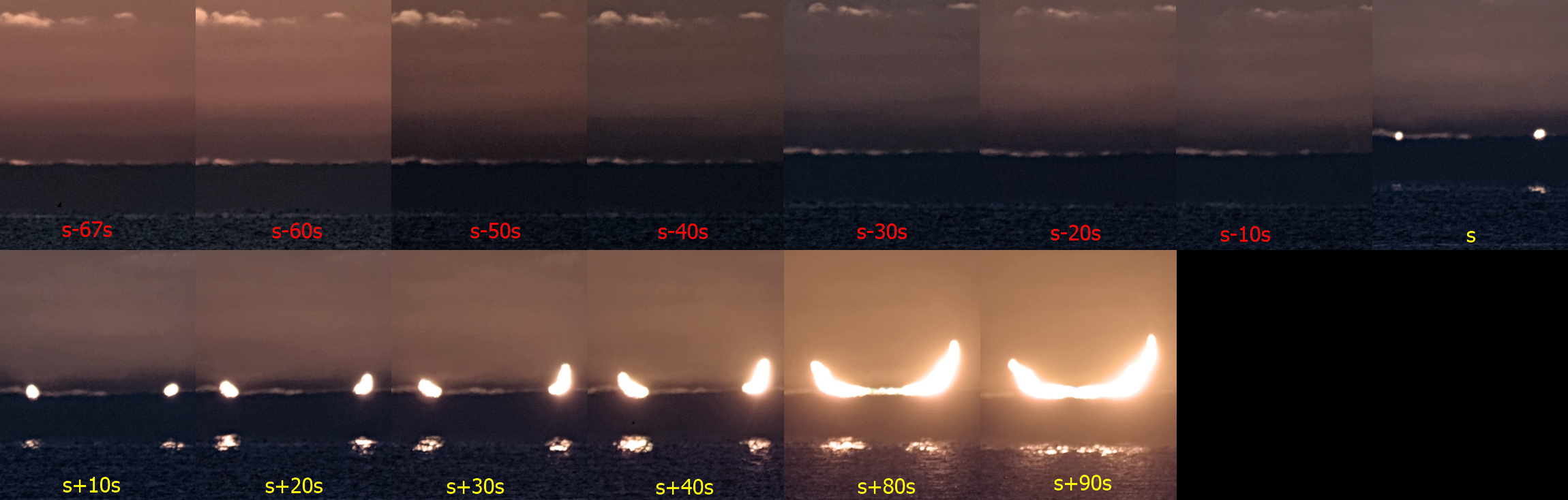
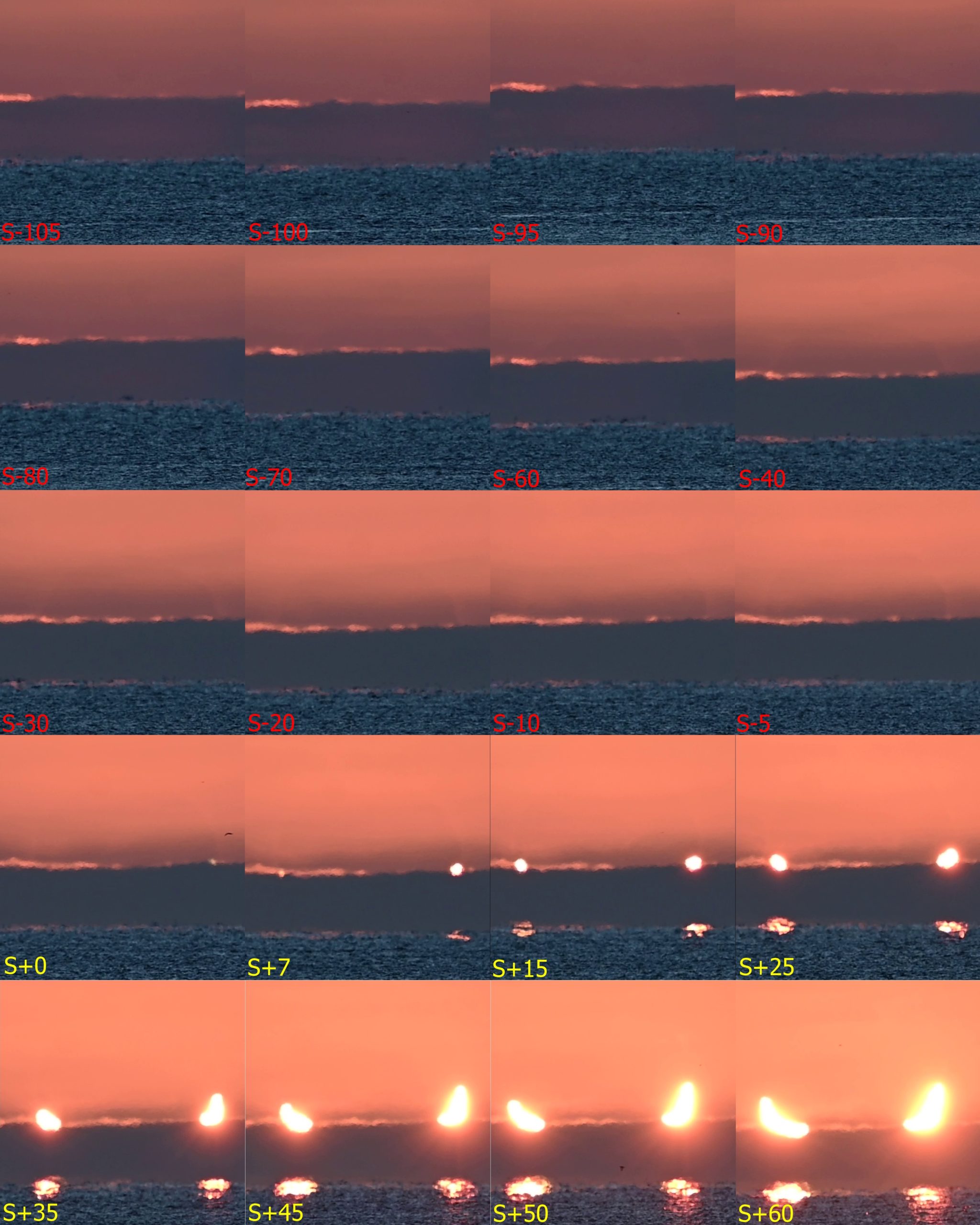
This was courtesy of another solar eclipse chaser, Mike Kentrianakis, who posted his observation on Facebook a day after Jason announced the corona visibility. He used the Canon M100 mirrorless camera with 55-200m lens. The results recorded by this device seem to look slightly better. Fortunately, by the way of awaiting the eclipsed sunrise, probably around the ephemeridal time, his video covered over 3 minutes earlier before the horns became visible. Thanks to this, we have the first “black sunrise” (or “black moonrise”) reported in history! The video screenshot sequences show the rising silhouetted Moon’s disk against the backlight of the corona. Initially, it’s not visible well, as it’s hard to determine the rough moment when the upper edge of the Moon’s disk becomes visible. This is an outcome of the non-ideal alignment of the Moon and the Sun, as we have the obscuration of 87%. The visibility of the lunar disk silhouette improves seconds later (Pic. 22).
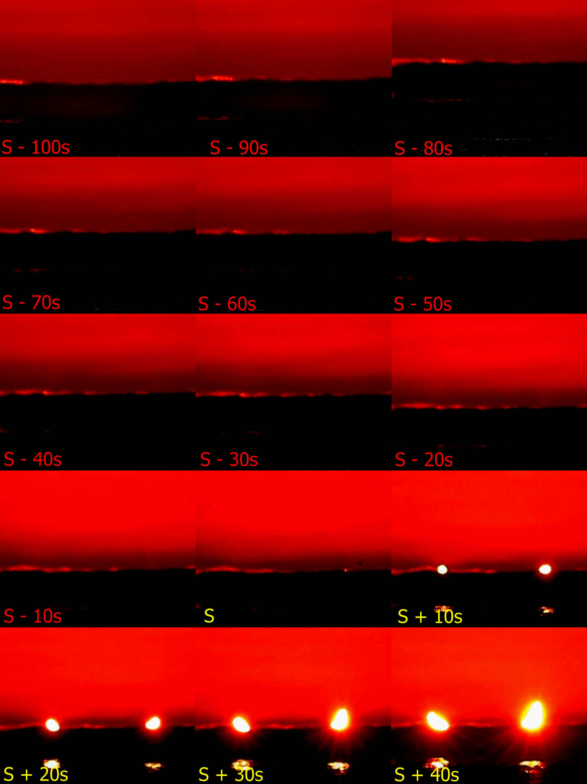
This report is more visible once the lunar disk projection is in place (Pic. 23). Unfortunately, capturing the moment the upper part of the Moon’s disk appeared above the clouds was impossible (S-90s). The brightness of the faint corona yielded the illuminated cloud edges, and a zone of higher humidity extended right behind them. Later, as the sequence shows, most of the “black sunrise” was reported quite well.
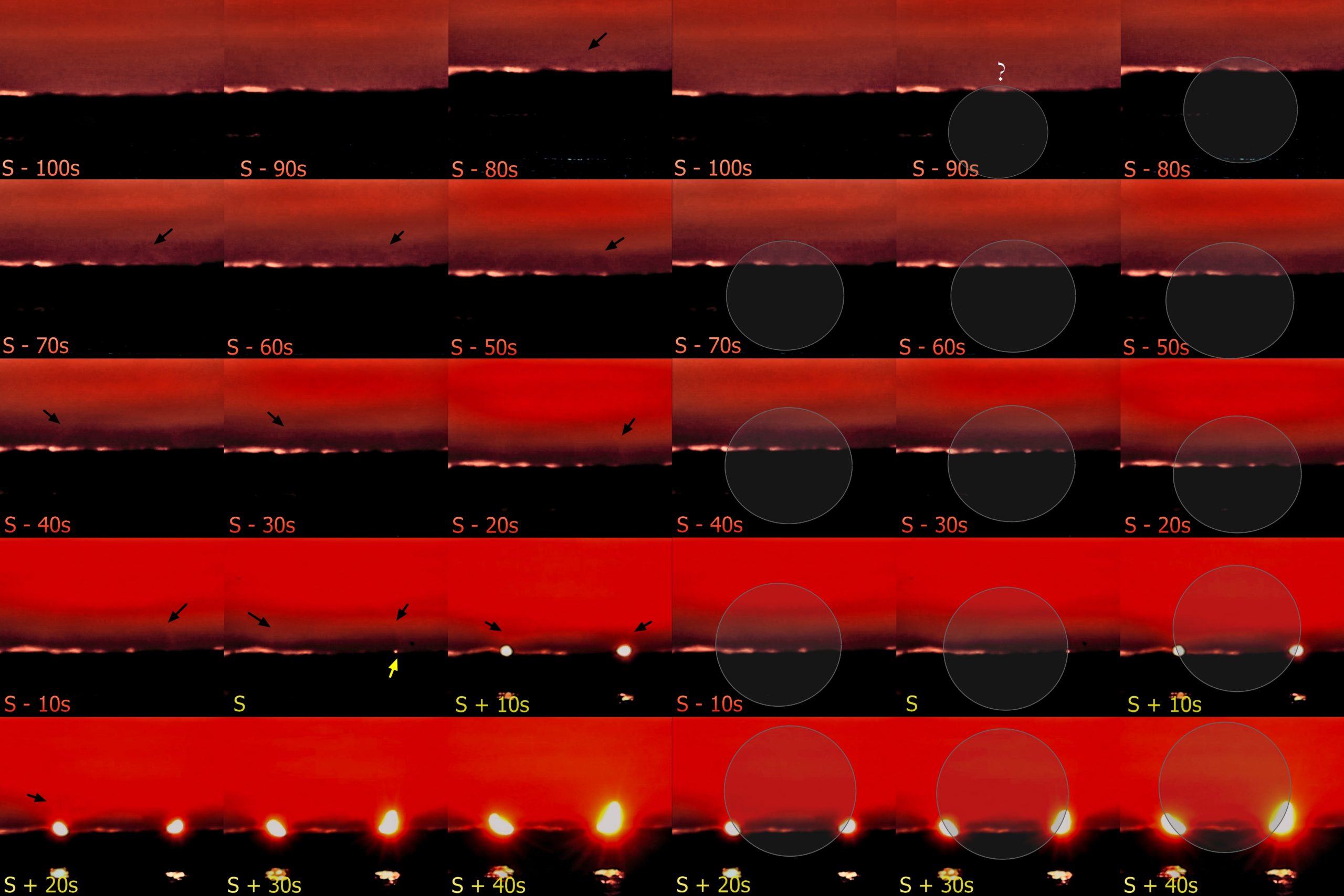
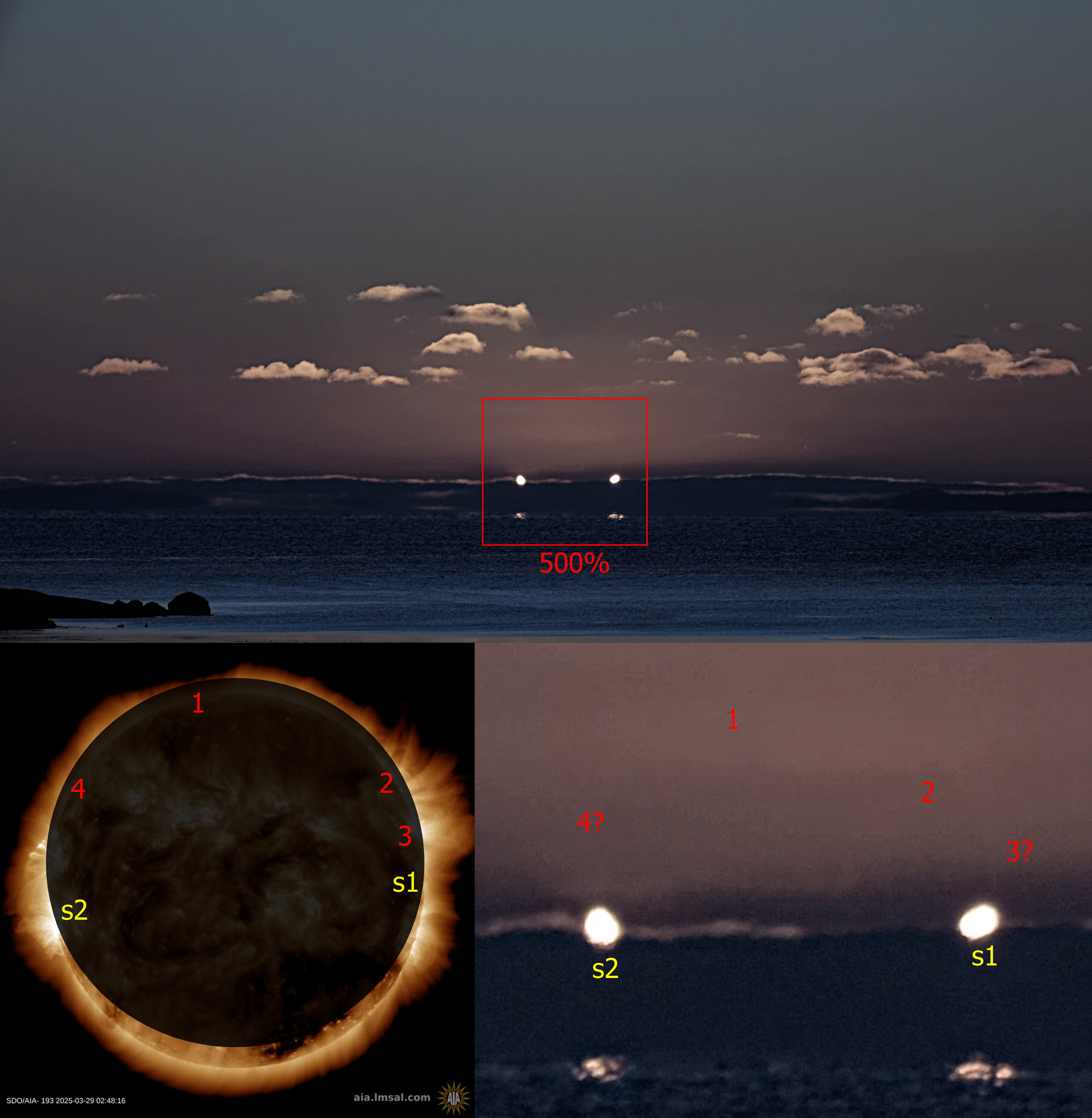
At last, I’ve considered the moments of best solar corona outline visibility (Pic. 24, 25).

The same optical elements as in the previous device can be identified now (Pic. 26 – 27).
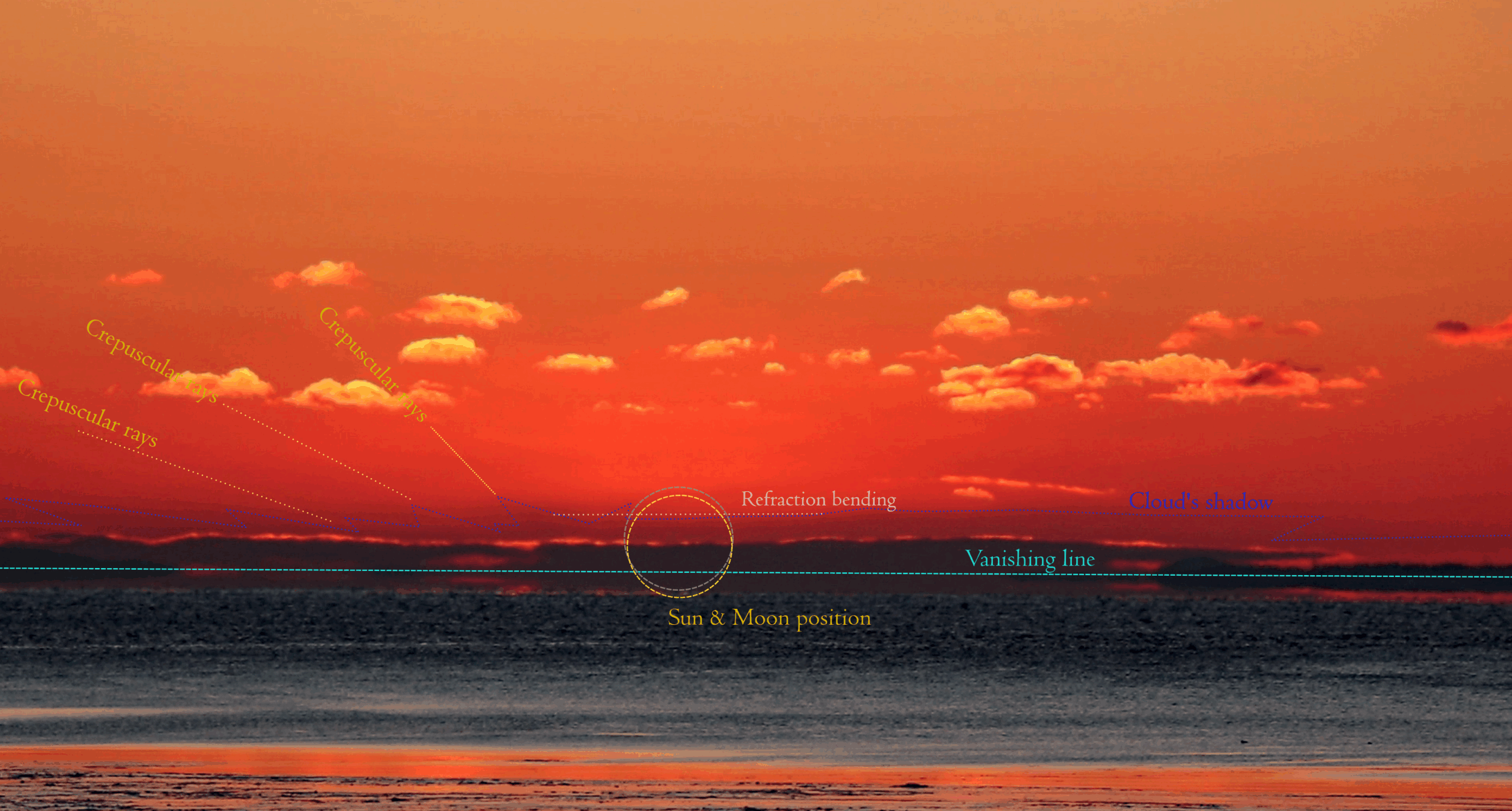
The last optical phenomenon that helped identify the solar corona outline was a slight refraction bending visible near the cloud’s shadow edge. The outline was slightly distorted (flattened) downwards at the indicated line. Looking at it from a different angle, the outline below the line was somewhat higher in the sky than it could be. The primary reason for it was the presence of a colder air mass beneath. Indeed, it was in place beyond the east bank of the St. Lawrence River, where the water surface didn’t alter the air properties. The Sun & Moon disk sketch represents their position behind the clouds, where the right horn was slightly higher than the left one, because the eclipse culmination was missed somewhat.
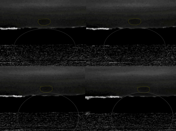
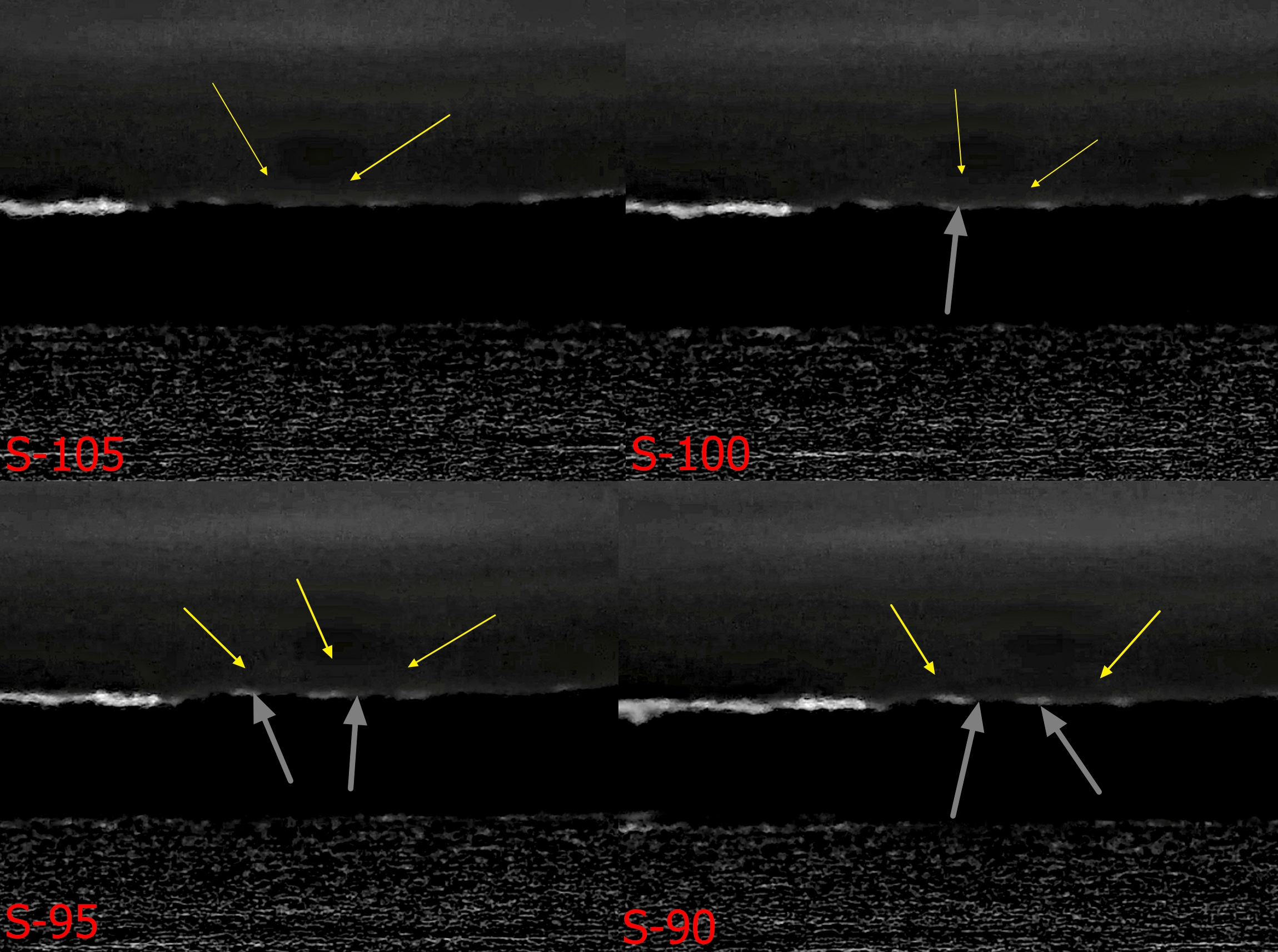
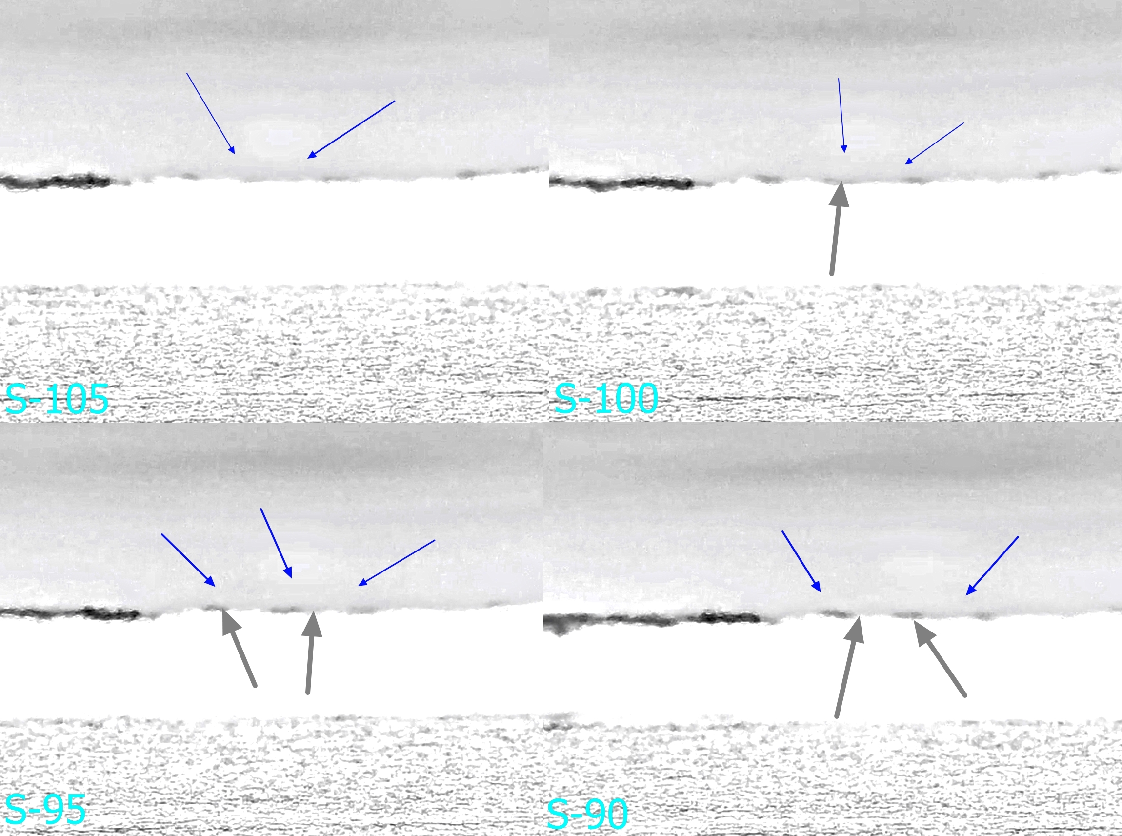
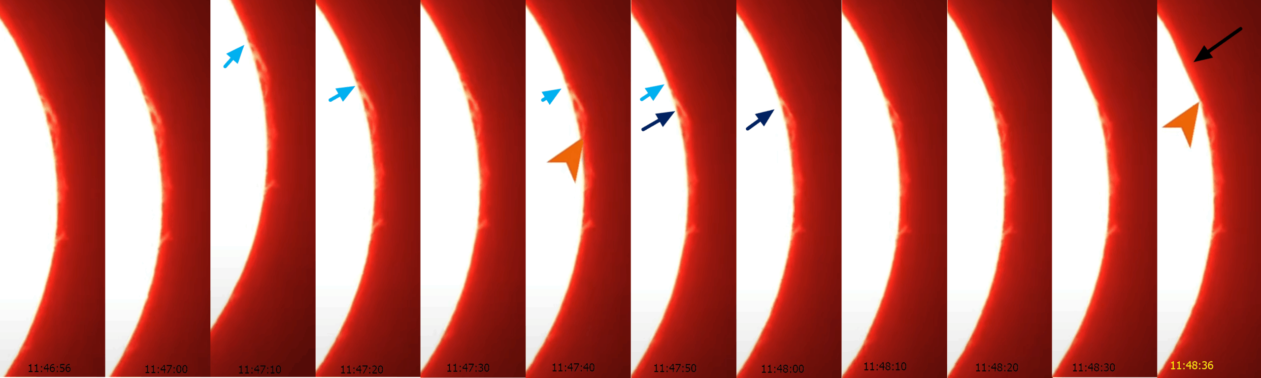
Usually, all the observers started to record their videos at sunrise, although the timekeeping in their devices could vary by a few seconds. Kevin Wood, with his equipment, Stock Nikon Z6ii with the Nikkor 180-600mm 5.6-6.3 VR mounted with the video parameters of 320mm, f/6, ISO 160, and 1/30s, was able to detect the exact moment of “black moonrise”! In his video, when S-105 marked 1m45s before the first cusp, the device detected some “weird fuzziness” just above the backlighted cloud deck. It doesn’t change the fact that the high level of humidity in that particular area hindered most of this faint light from passing through. Later sequences show that the “fuzzy arc” rises (Pic. 28-29, 32-34).
On the other hand, the faint solar corona disappears completely at the time of S+50 from the Stock Nikon Z6ii’s camera perspective. However, the horns were too dazzling for observers to see them with the naked eye.


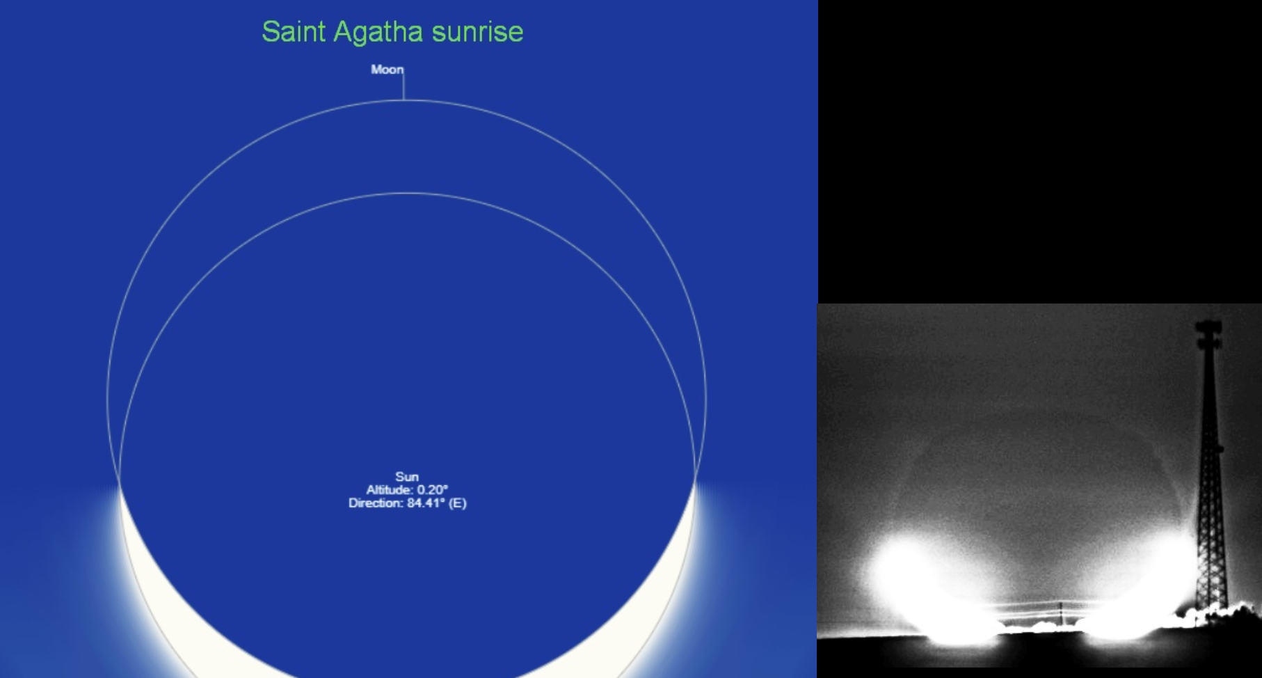
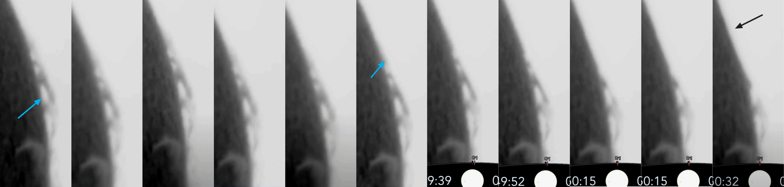
As mentioned earlier in this chapter, there are not only records of faint solar corona. Another observer, Vinod Kumar Vijayakumar, captured the “Black moonrise” from within the US borders! The Lakeside View restaurant at St. Agatha was a good spot for an eclipsed sunrise, with only 85.9% of the sun obscured (Pic. 36). His images appear to be the best because they are DSLR images instead of 4K video screenshots (Pic. 28).

Like above, the corona outline disappears several seconds after the Sun’s crescent becomes visible. The weather conditions at St. Agatha were similar to Les Escoumins, so the description above applies to this observation. Thanks to the deep analysis made by Dan Fisher, we can see a highly contrast-enhanced image of the solar corona (Pic. 37).
Let’s have a look at more detailed solar corona observations. More detailed observations can be found at this link, but the archive update is about a month behind. Therefore, there was no option to perform analyses right after the eclipse day. On the day this section was produced, I could capture the image of solar corona at the exact moment of “black sunrise” visible from Les Escoumins (Pic. 38).

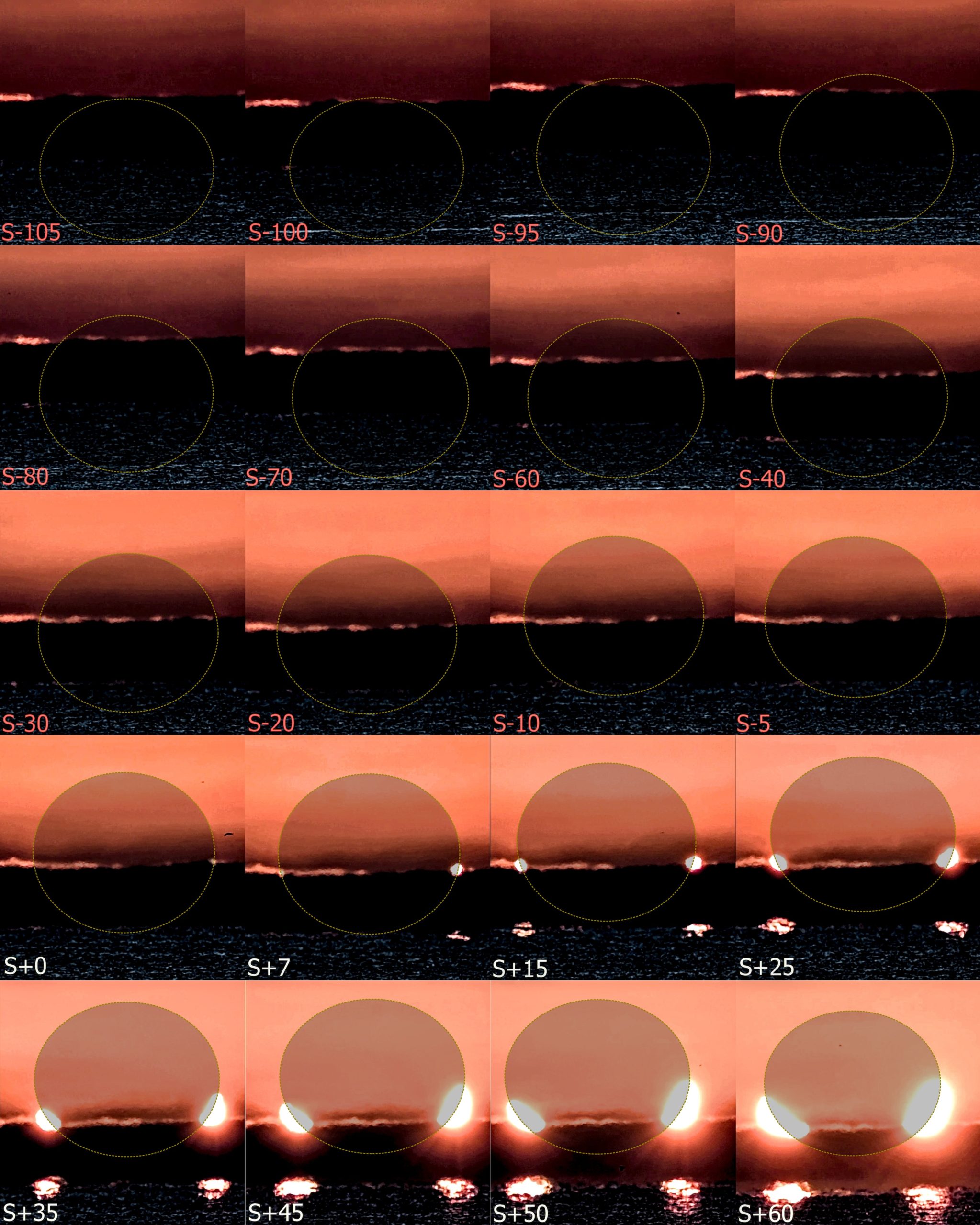
Now, we need to model the obscuration of these images based on the eclipse circumstances. The photo below (Pic. 40) presents the Moon’s limb movement across the Sun during Jason Kurth’s video time until the corona outline disappears (Pic. 14).
Another images visualize the position of the Moon’s disk at the moment when the horns rise above the clouds (Pic. 40)

The last images (Pic. 41-42) show the solar corona visualized in all models simultaneously, including the Moon’s position and indication of the brightest elements visible to the observer (device) at the moment of the “black sunrise.”
3. DEVIL’S HORNS FROM VARIOUS PERSPECTIVES
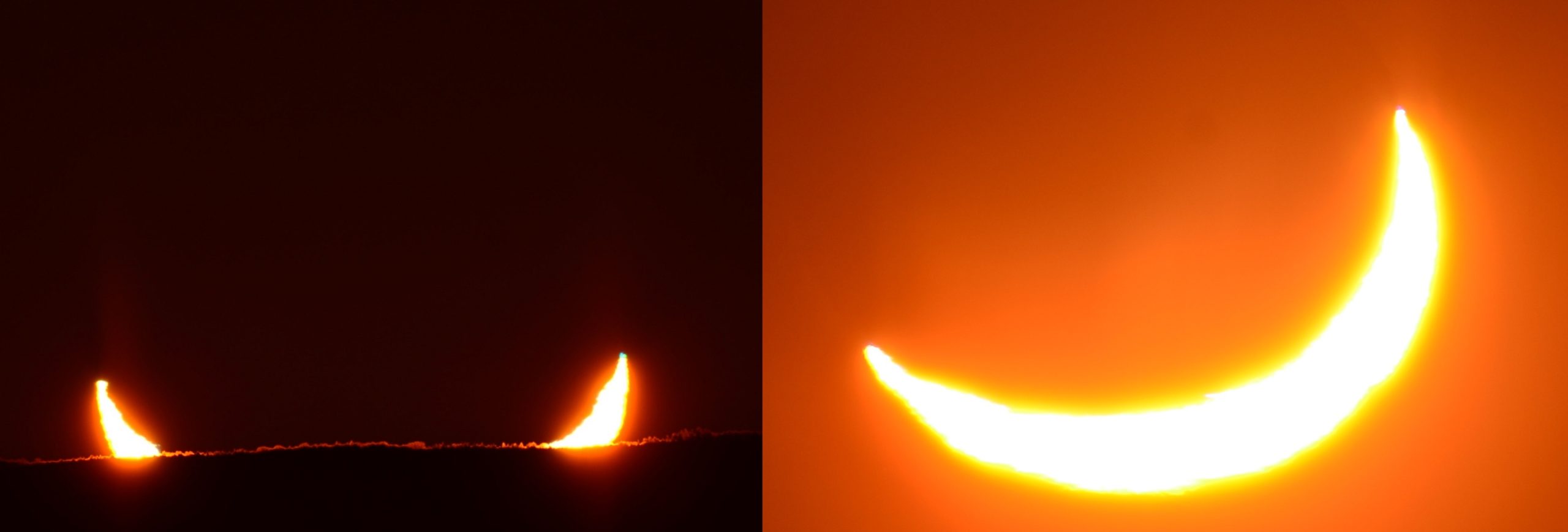
Viewing the Devil’s horns is the most common purpose of travelling to watch partial solar eclipses. They look more effective as the eclipse phase is deeper. The name “Devil’s horns” comes from the specificity of the phenomenon. The rising (or setting) Sun is predominantly orange or red due to light extinction in the Earth’s thick atmosphere. The second reason is the upright orientation of the solar crescent, which, when rising, reveals two separate horns looming at the horizon. This background is pure geometrical and well explained by the sketch below (Pic. 43).
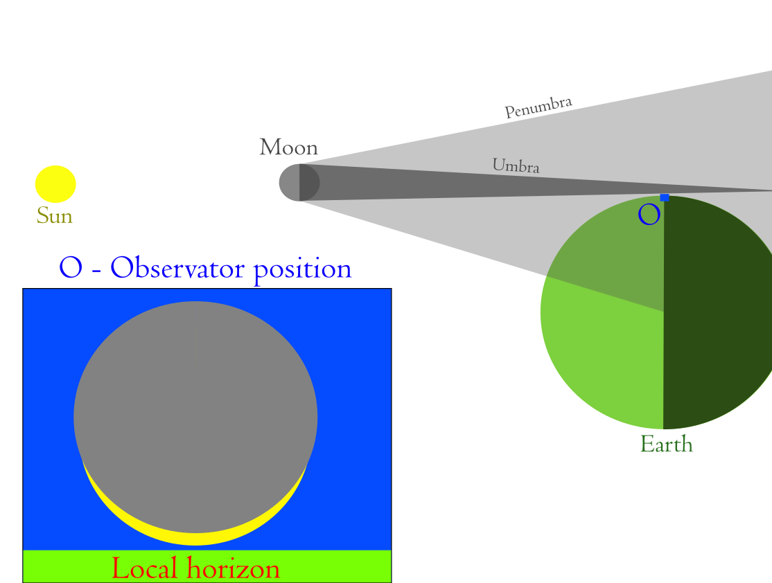
The Sun’s crescent is always oriented straight up. It’s an effect of imperfect alignment of the Sun and Moon, in which the umbra misses the Earth’s surface at a closer or farther distance. Regardless of the hemisphere or the umbra position against the Earth, an observer standing at the point where the greatest eclipse takes place will always be placed somewhat “underneath” the lunar shadow column, which passes somewhere above his head. In light of this situation, the Moon’s disk is placed slightly above the Sun’s disk, making the crescent visible. An analog situation can occur just beyond the geometrical path of annularity, or totality, when the umbra is adjacent to the ground, but doesn’t “touch” it at all. When considering the partial solar eclipses only, the Devil’s horns can be observed geometrically along the entire line of the terminator until the magnitude of the eclipse is too low for the crescent appearance. The deepest eclipse in the given moment will always occur roughly at the geometrical moment of sunrise, including refraction. The “ideal” and the deepest magnitude occur when the center of the Moon’s disk coincides with the geometrical horizon line. Practically, the Sun’s horns up might not be visible to the observer at that moment, because when the eclipse is deep enough, they are just underneath this horizon line. Another matter is the symmetry of the solar crescent against the Moon’s disk. We can talk about the most significant eclipse phase at sunrise or sunset only when the two cusps appear or disappear simultaneously. It’s not trivial to capture, as the entire Moon’s disk is in motion. The essence of this aspect is shown in the sketch below (Pic. 44).

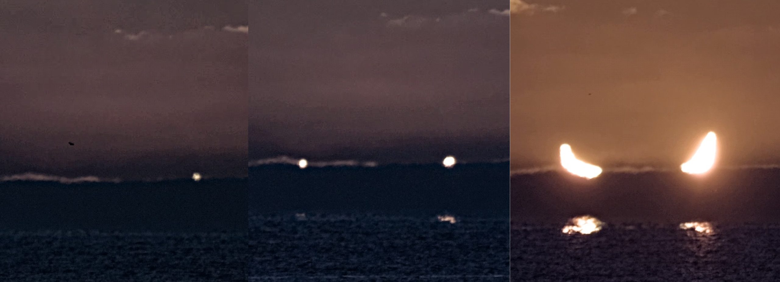
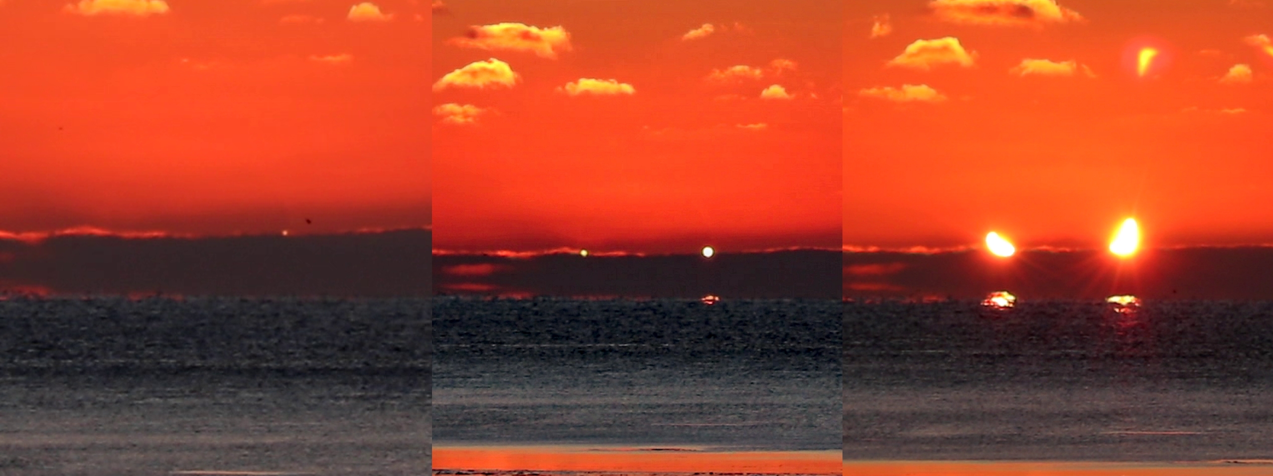
Most observers report the sunrise/sunset in cases I or III. Even both observations reported above don’t capture this “ideal moment.” For both observers, from whom I got the videos, the Sun’s first appearance isn’t symmetrical, although this is the closest moment I have ever seen. The right horn rises around 10s earlier than the left, which means that the greatest eclipse was slightly missed out, due to the distant cloud deck visible at the horizon (Pic. 45, 46).
Similar eclipsed sunrise circumstances were captured from Maine, US (Pic. 47), even with the green rim optical phenomenon, typical for the situation where the local atmosphere has quite a high humidity level. As it has been said, the weather conditions described for Les Escoumins could also be applied to northern Maine, where they were similar.
The most ideal conditions of symmetrical “devil’s horns” were reported from St. Agatha village (Pic. 48).

Now let’s see a few images taken at sunrise, but shortly before the maximum occurrence. The closest moment to the maximum was covered by Pam Greene Hobbs, where we can see left horn slightly up against the right one. The eclipse culmination was about to occur a while later (Pic. 49). In the same situation was Edder Carrillo, who was watching the eclipse event from Caribou in eastern Maine.

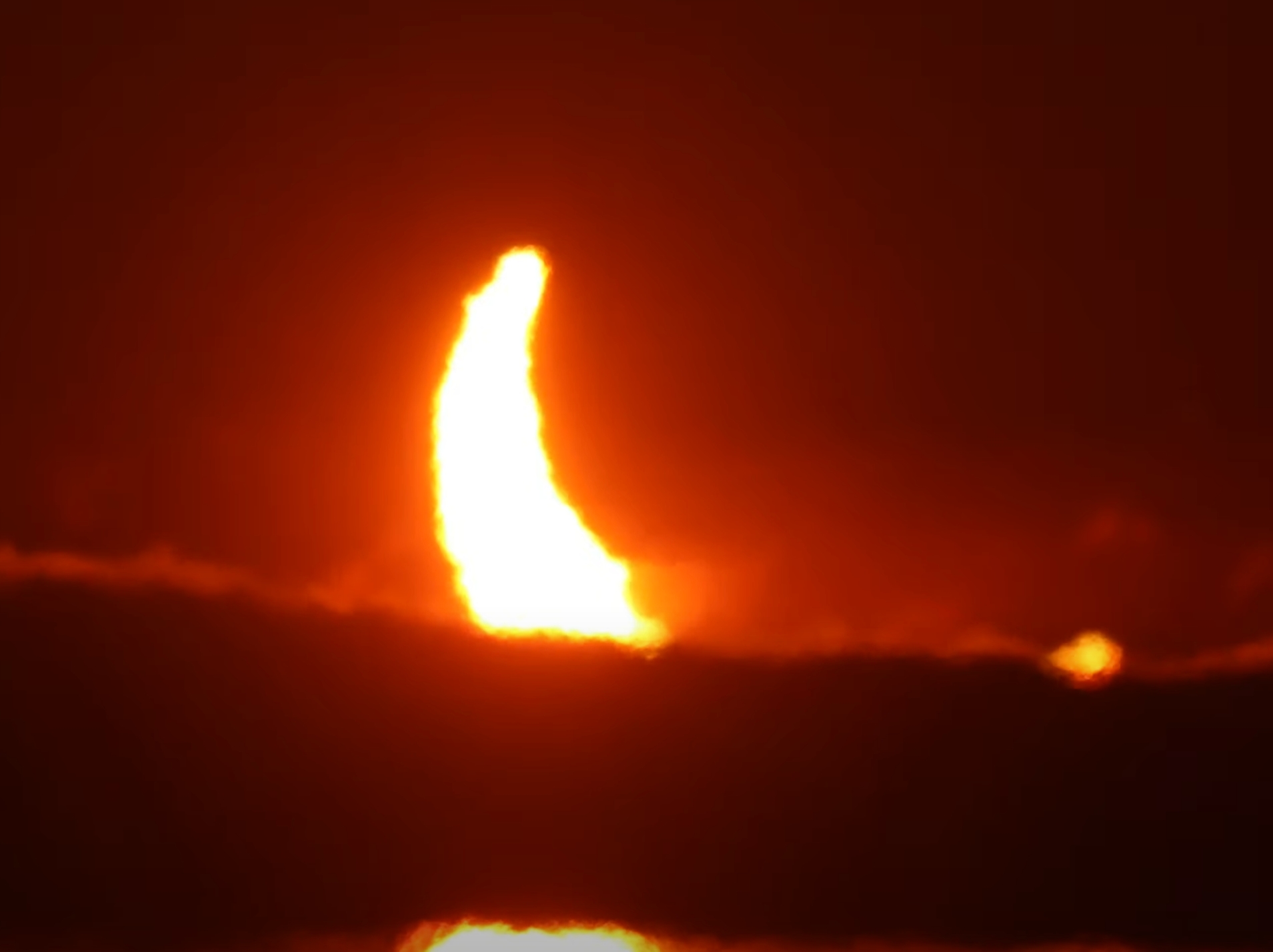
For those watching the rising “devil’s horns” along the St. Lawrence River, but located more northeast, the crescent was more asymmetrical despite greater magnitude at maximum. The light from the rising crescent passes at too low an angle across the warmer layer and is refracted. For the observer, the light from the upper part of the crescent appears to be coming upwards from the horizon, and the observer’s brain interprets it as the reflection from water. The horizon line is missing, which is how the vanishing line effect looks. The Sun’s crescent at sunrise is somewhat duplicated against the invisible “line”. Pictures below show exactly the effect (Pic. 50, 51).

The eclipsed sunrise was watched through the much warmer air the St. Lawrence River heated. At least in Les Escoumins, we estimated the difference to be 18 degrees Celsius. As a result, regardless of the level of optical zoom used, the heat shimmer (or heat haze) is omnipresent. This is an effect of air convection produced by a vast difference between warmer air beneath and colder and much denser air above. This difference causes a gradient in refractive index, which produces this shimmering effect.
For these two places shown above, the obscuration reached 87,7-87,8% at maximum, but because the entire crescent was up, the corona outline was invisible.
Finally, we can consider simply the eclipsed sunrise, at which the devil’s horns’ appearance isn’t obvious, and can be assigned only to the area with rough topography, where mountains or hills prevail. In such a situation, the maximum eclipse can be observed above the geometrical horizon. In contrast, the crescent with both horns up will rise or set behind some hill. For better understanding, we can look at the images below (Pic. 54). This situation will be related to scenario I (Pic. 44) when the greatest eclipse is observed after sunrise, and conversely, scenario III in the case of sunset. In this situation, we can say that “false devil’s horns” will appear only in favorable local topographic circumstances but never against the actual horizon.
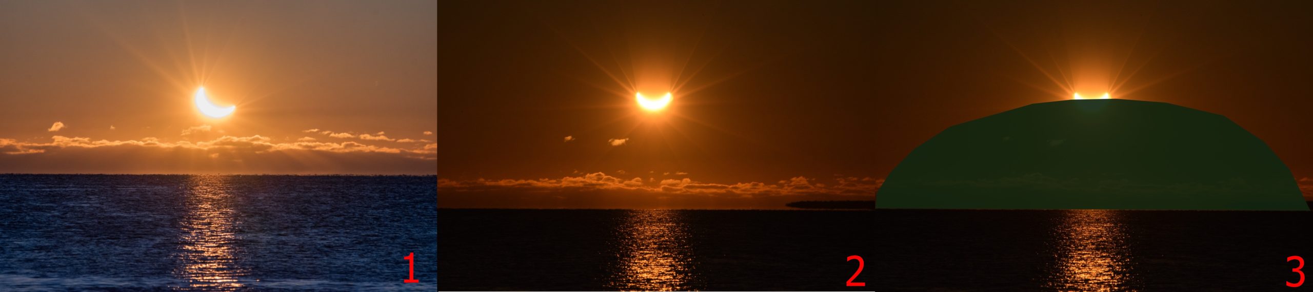
The solar crescent can be oriented even vertically at sunrise, but as the eclipse progresses, it changes the orientation (1), with both horns up at maximum (2). When the crescent rises (or sets) already behind some hill (3), it can appear as “false devil’s horns.” Situations such as this will apply to all partial eclipses, even those that occurred along with central ones observed on Earth.
4. IMPACT ON TWILIGHT REPORTED BY THE WEB CAMERAS
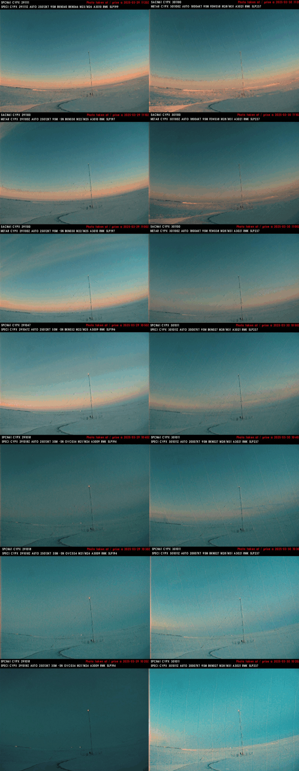
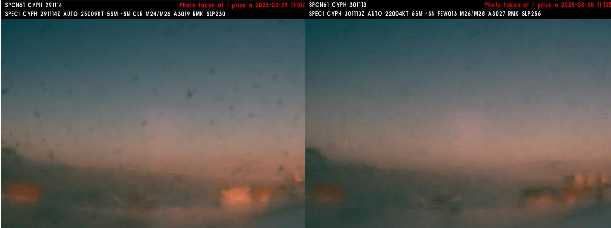
The deep partial solar eclipse in Canada could be observed remotely by courtesy of the Digital Aviation Weather Camera Website, a nationwide provider of meteorological cameras with a refreshing mode once every 10 minutes. It’s a poor frequency as far as solar eclipse events are considered, but at their worst, these cameras are basic themselves. Their small resolution and sensor didn’t allow for any optical analyses of the differences in light level expressed by significant ISO sensitivity variations. There are three places on the east bank of Hudson Bay, where the webcams are mounted in three or even four directions. Because the results aren’t competitive with webcam-based reports made by previous eclipses, I will place them just one by one (Pic. 55-56, 58-61).
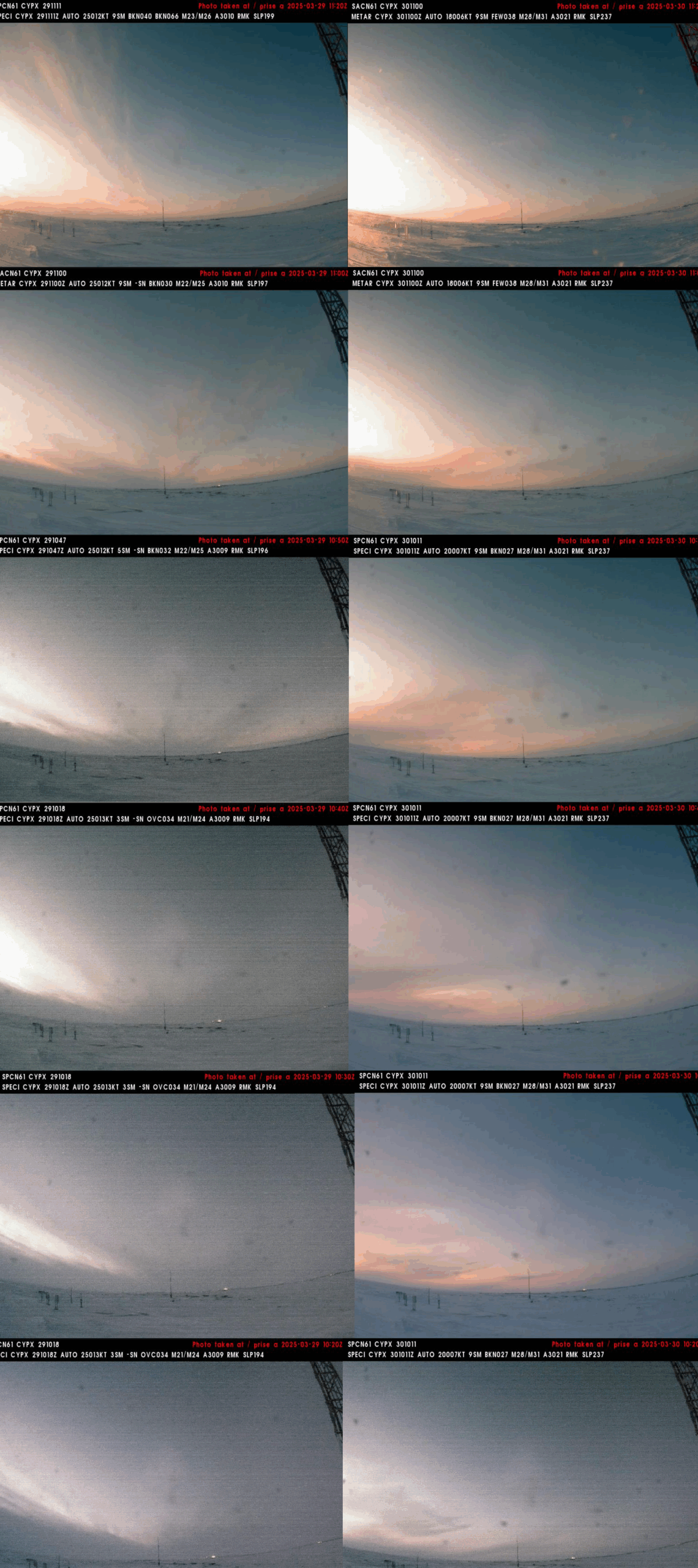
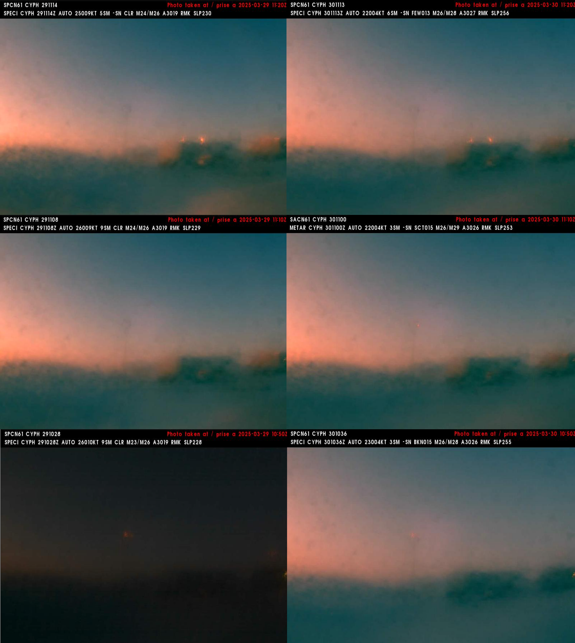
Puvirnituq weather station was the closest to the greatest eclipse point, located east of Akulivik. The webcams show local weather conditions with clear sky and good visibility of the receding twilight wedge. The changes of coloration in the sky and the scene are barely visible. The webcams show significant dynamic in the ISO sensitivity changes ass the eclipse progressed. The impact of this eclipse on civil dawn is expressed well at all moments. At 10:20 UTC, the eclipse magnitude was about 0.5 at that location. Twenty minutes later, the obscuration exceeded 83%, giving the reddening Earth’s shadow a strong, dark appearance. Later, when the eclipsed Sun was up, paradoxically, the left image sequence shows a brighter scene than usual. This is the aforementioned variation of ISO sensitivity due to camera auto-adjustment to the illumination conditions. What is, indeed, the most important is that the SE camera shows the overcast eastern section of the sky through high-level clouds. Observing devil’s horns with much better expressed solar corona at obscuration of approximately 93% wouldn’t be possible, though. The altostratus and cirrostratus clouds were prevailing at solar azimuth. The eclipsed Sun became visible several minutes later.
Considering the overall light level changes across the whole eclipse event, the maximum indicates the darkest moment at once. This trivial thing isn’t quite evident when the scene faces quick brightening or darkening, which is typical around sunrise or sunset. The coincidence of the darkest moment with the maximum eclipse results from the overall illumination changes and the level of eclipse obscuration. Looking at the chart below (Pic. 57), we can see the impact of this partial eclipse on twilight and golden hour. The around-sunrise period marked the most noticeable difference. For Puvirnituq and Akulivik, the crescent sunrise resembled the illumination conditions similar to early civil dawn, when the non-eclipsed Sun is around 4 degrees below the horizon.

Surely, for Akulivik, the “darkest” moment is explicitly shown, whereas it doesn’t exist at all for Les Escoumins. There are two essential reasons behind it. The first one is undeniably the eclipse obscuration, which coincided with quick illumination level changes around sunrise, will cause this effect, or simply not. The strict threshold hasn’t been investigated yet, but the moment exists for obscuration of 93,1%. The obscuration of 87% at Les Escoumins wasn’t enough for an effect such as this, and instead of it, the dawn progress was slower than usual. Another culprit is the latitude. The difference of approximately 13 degrees in latitude is translated into the angle at which the Sun comes up at the horizon, and thereby the length of the dawn & golden hour period. Since Les Escoumins is located further south, all these twilight-related phenomena occur faster than in the north. In turn, the impact of the eclipse itself is less pronounced. On the other hand, the eclipse at these latitudes fits almost the entire twilight period in a geometrical sense, unlike the other location where the eclipse progress is relatively shorter than the twilight period. At Les Escoumins, the dawn just slowed down, and observers flocked to watch the eclipse, which would appear as if the Sun would be around 1,5-2 degrees lower beneath the horizon than normal (Pic. 57, 58).
Despite the shallow solar depression, the streetlight could cast shadows, typical of early civil dawn. This article explains more about this.

At Kuujarapik weather station, the greatest eclipse occurred at late civil dawn, when the Sun was 2,5 degrees below the horizon. The impressive obscuration of 91,5% went unnoticed due to poor webcam quality. The shot taken at 10:50 UTC looks intriguing. The snow probably catches the first beams of the crescent sun. However, this location wasn’t proper enough for watching the devil’s horns.

The Inukujak weather station provided the worst webcam, but we can see a clear sky except for the eastern horizon. The conditions could be similar to Les Escoumins, but the obscuration was 92,7% at a solar depression of just 1,4° when the maximum occurred. With the obscuration of about 91% and strong asymmetry of Devil’s horns, the chance of seeing the faint solar corona was high.
5. SUPERB RECORD OF “CONTACT 0” FROM POLAND
The entire solar eclipse event includes four contacts, as far as the central path is considered. An observer can effectively see the 1st contact, when the Moon’s disk “touches” the solar limb, the 2nd contact, at which totality or annularity begins, and consequently the 3rd and 4th contacts representing further eclipse progress in reverse sequence. However, exceptions are reserved only for observers equipped with the H-alpha instruments, who can understand the Sun’s surface structures, especially those extending outward from its surface like prominences. In my previous text about solar H-alpha observations, I mentioned some basic information about the typical height of prominences, which is estimated at 100000km (Mackay, 2021). However, in some exceptional cases, they can reach an altitude of 5 or even 8 Mm. In light of these circumstances, we shall mention two additional “contacts” reserved for the H-alpha equipped observers, who can see when the lunar disk starts to cover the prominences before it approaches the solar limb. This is not a rule, as the prominences don’t appear at the entire circuit of the solar disk. This particular moment should be called the “contact 0” as opposed to the “contact 5th“ in converse circumstances at the end of the eclipse event. In my hometown, we tried to catch them on June 10, 2021, during a small partiality, but they were visible on the other side of the solar disk when the 1st contact occurred. This, such a common thing, isn’t subject to direct H-alpha eclipse observations. The best proof of it is a myriad of YouTube & Vimeo videos, which show partial solar eclipses in H-alpha just between the first and last contacts, or even shorter. Despite the multitude of instruments located worldwide, I wasn’t fortunate enough to see the “intention” of covering the periods shortly before the first and after the last contacts. For a detailed estimation of the “contact 0” at least for the location, which falls within the umbral or antumbral path, we need to know the angular speed of the Moon in the sky. Being more precise, against the Sun, towards which the Moon always has positive acceleration. It explains why the Sun always starts to be bitten from the “right” when watching the event from the umbral path. It’s another topic for further texts. For the angular speed of the Moon, we can use the value of 0.37″/s, which would give us 22,2″ per minute. If the typical solar prominence has an angular altitude of 0° 2′ 19.34″, then the time between the “contact 0” and the 1st contact could be almost 6m30s. However, it would apply only when the Moon heads toward the solar prominence centrally. As in many cases, the Moon doesn’t head ideally on the prominence, this time span will be shorter. On two observations made in Poland, where the eclipse magnitude was about 0.15, we can see that the “contact 0” is observed around 1-2 minutes before the solar eclipse begins (Pic. 63, 64). We must be aware that all the estimations above have a general character, which applies also to the mean Moon-Earth distance, whereas the Moon on eclipse day was closer.
I guess it might be the world’s first observation of the eclipse this way, which has been made intentionally with full awareness of the phenomenon. The H-alpha approach, proposed on this occasion, is excellent for situations like this and for grazing eclipses at a specific place just next to the penumbral limit. Additionally, the article explains the other circumstances under which observations such as these can be performed. Chasing “contact 0” or awaiting “contact 5th” can be great outreach for any solar eclipse, even for the locations directly neighboured with the penumbral zones, at which the lunar disk can occasionally graze the solar prominences without “touching” the Sun’s disk at all.
6. LUNAR TOPOGRAPHY DISPLAYED ON PROJECTION METHOD IN MY HOMETOWN
The optical projection is an easy and safe way to get a good image of the Sun on a plain-coloured surface. This surface can be white paper or board. Depending on the distance to the instrument, the image of the partially eclipsed Sun can be enlarged. The spectacle projection, which was used at the Leszczyński High School astronomical observatory in Jasło, is one of the best for partial eclipse observation. The spectacle projection can be done with the telescope or binoculars. However, the biggest flaw of this method is the quick heating up of the mirror or lens by warm air coming between the lens and the eyepiece. In extreme cases, the mirror can be misshapen, resulting in image deterioration, or the device can be damaged entirely by melting down some components. It’s good to have the telescope specifically dedicated to solar observations only. This method allows observers to see the sunspots on a bigger, brighter, and sharper solar disk. When watching the partial solar eclipse, we can see the lunar topography in a sharp image projected on the board (Pic. 65 – 68). Unless this observation doesn’t take long, we will be fine with the telescope components.


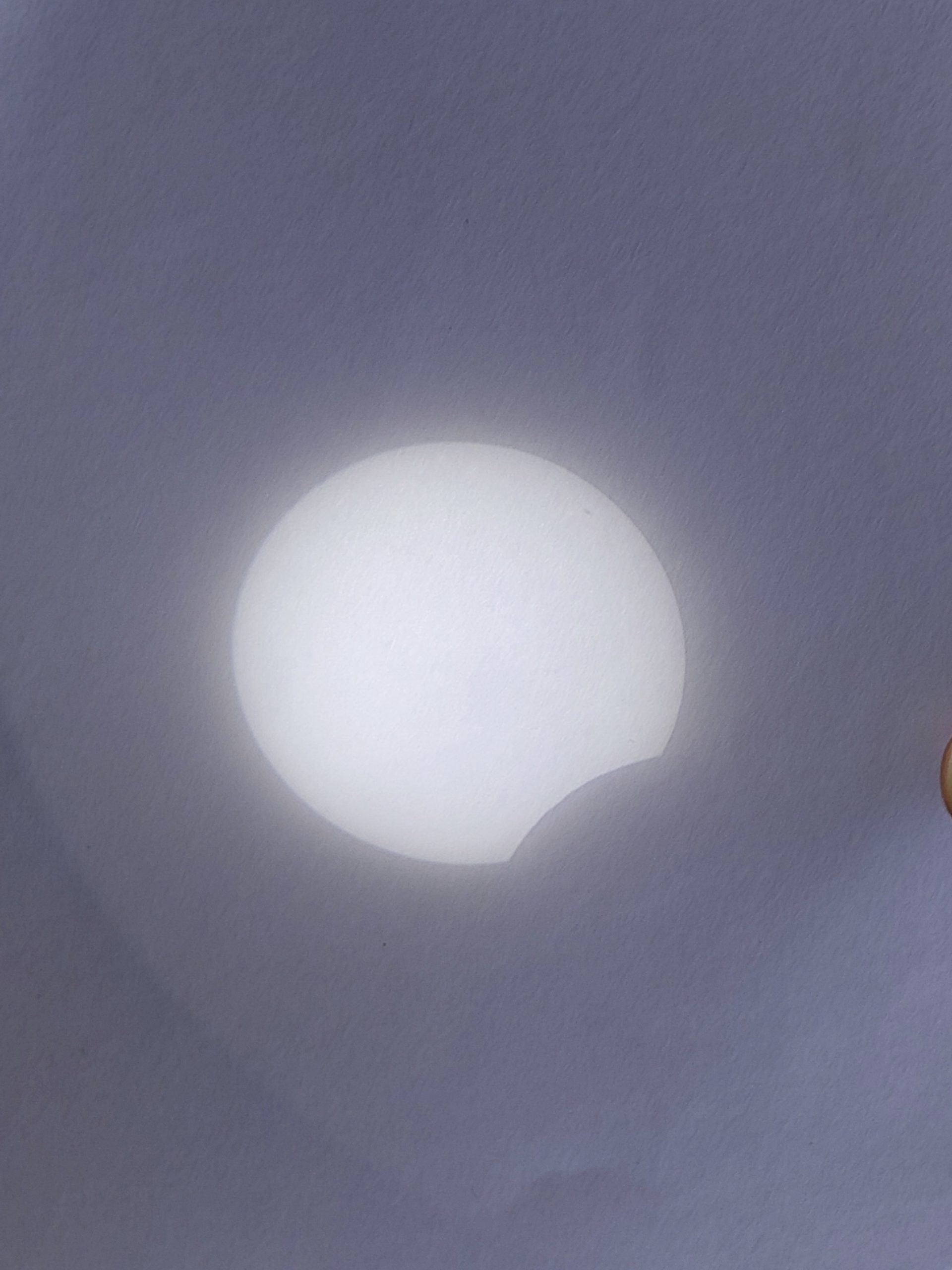
We were pretty unfortunate with this observation, as high-level clouds veiled the Sun. As a result, the image isn’t as sharp as it could be. The sunspot of 4046 was visible too (Pic. 69).
7. THE REDDENING OF SATELLITE IMAGERY EXPLAINED
Satellite imagery near the umbra of solar eclipses can dramatically document the reddening of the clouds. Usually, the effect is visible well for areas with magnitude exceeding 0.50, at which the very center of the Sun is no longer visible, and the limb darkening effect starts to prevail. Of course, it doesn’t happen abruptly. The effect increases gradually along with the increment of eclipse magnitude. The best view of this effect on satellite imagery is provided by zoom. earth service, where anyone can see the real-time view with several hours of backup. This service is based on NASA high-definition, which comes from NOAA, GOES, MODIS Aqua & Terra, and others, and shows the image in true coloration. MODIS “true color” images, which have three channels of visible light, are designated to show how the surface top clouds would appear to observers standing or flying immediately overhead (Gedzelmann, 2020). The images are processed with an algorithm, which removes the effect of Rayleigh scattering between the Earth’s surface and the top of the clouds and the satellite. Additional coloration of surface features can arise from scattering and absorption caused by various aerosol particles like smoke plumes or haze. When they aren’t elevated and don’t affect the cloud coverage above the given area, the clouds, similar to snow coverage, appear white. The cloud-top colour is height-dependent, the lowest cloud deck will express the most significant shift towards red or even brown. The deeper red or brown tint will also be observed in the areas closer to the umbra, where the light comes only from a thinner outer sliver of the solar limb. In this situation, the light comes somewhat from near the top of the photosphere where the temperatures are as low as 4400K. The impact of the proximity to the umbra is expressed by the range of tinges from yellowish at the magnitude of approximately 0.50 to dark salmon-brown in the direct neighborhood of the totality.
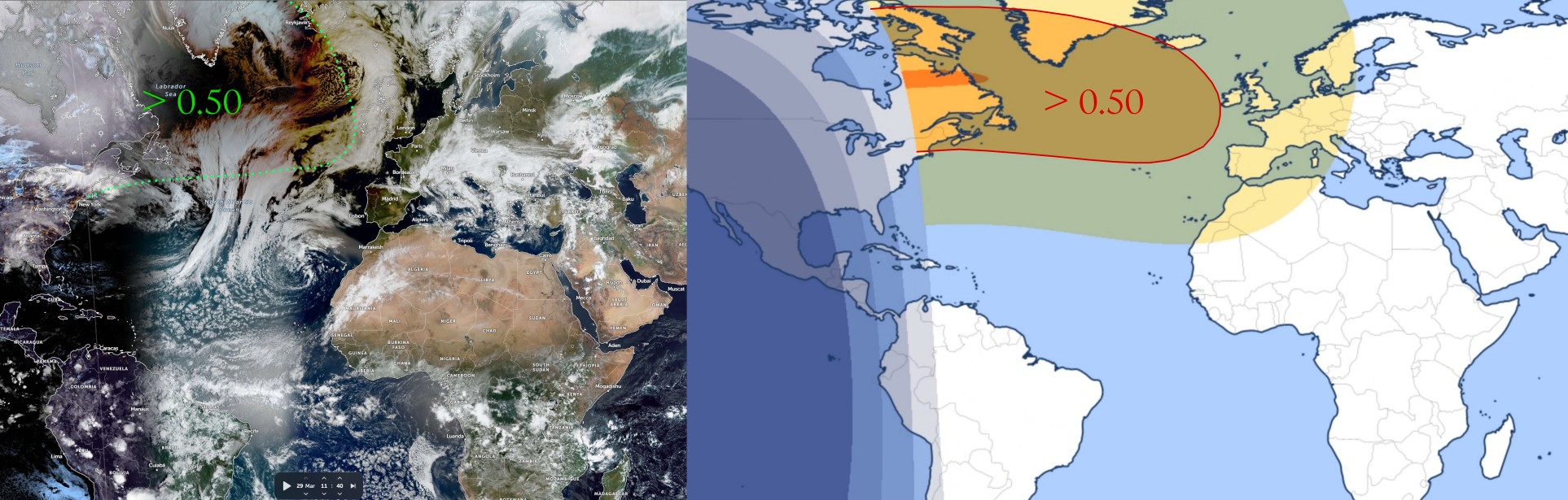
The description above represents the simple case away from the terminator line. However, the partial solar eclipse of March 29, 2025, sticks to a quite opposite situation, at which theoretically, the dark salmon-brown tinge could be visible right above the north Quebec area. The Sun was too low for the satellites to detect its beams. If the terminator line weren’t marked, we could guess it’s still nighttime or at least twilight. Theoretically, more detailed imagery could be available from worldview.earthdata.nasa.gov, but they make updates separately for different regions at different times. The effect can be visible only in places (Pic. 71).
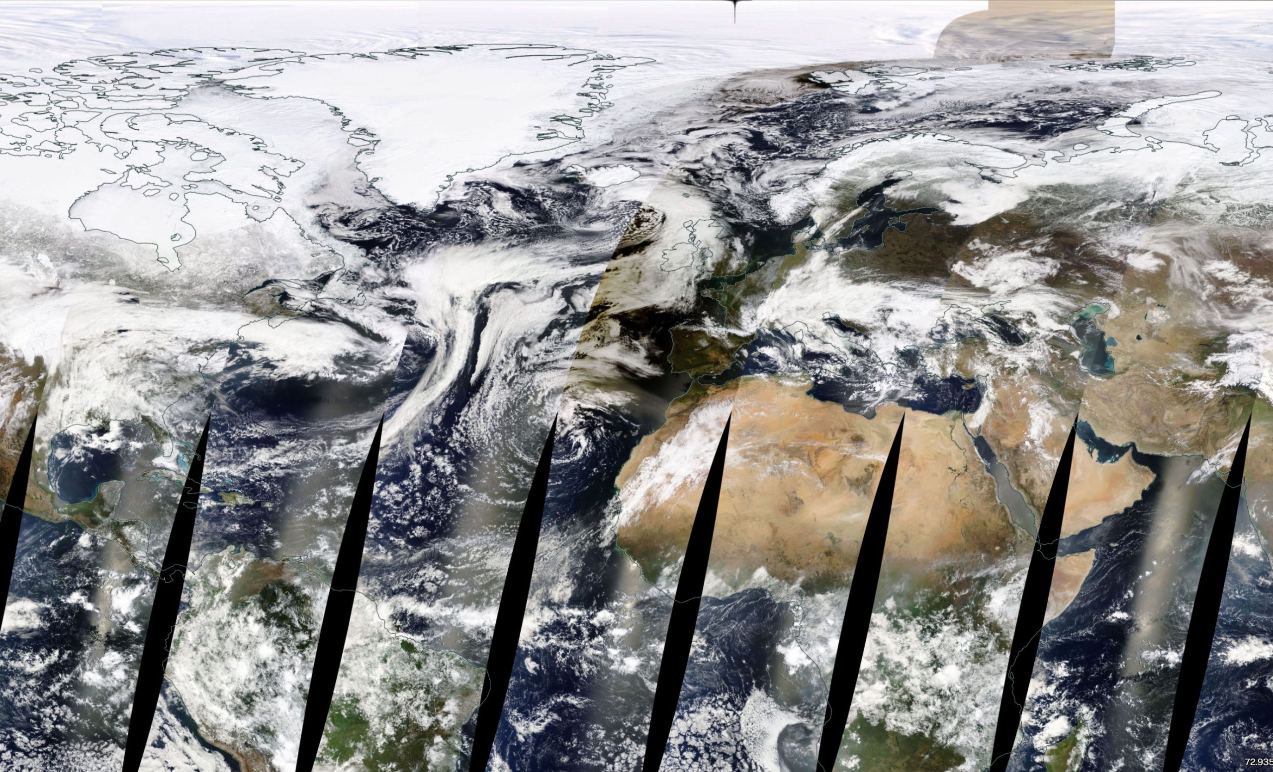
The view of the eclipse’s impact on the cloud deck coloration changes as the eclipse progresses against the time of day. This is best visible in the animation below (Pic. 73).

The reddest top clouds and surface will occur in the following conditions (Gezdelmann, 2020):
– proximity to the horizon,
– proximity to the umbra,
– when the Sun is lowest in the sky,
– when the cloud top is lowest in the troposphere,
– when viewed from a great height above the cloud top or surface.
The analysis of cloud top coloration in solar eclipse conditions is an innovative approach to determining the vertical temperature gradient in the solar photosphere.
8. CONCLUSIONS & SUMMARY
The text explains how to understand the geometry of a partial solar eclipse by understanding it as a non-central type on the Earth’s surface. The geometry and relevant computations determined the shortest distance from Earth’s surface to the umbra from two locations. The first location is where the greatest phase could be observed; the second location is where at least a few people observed the eclipsed sunrise. The computations also concluded that the sky above the observer’s head was darker at the greatest phase in both locations. A partial solar eclipse’s essence is understanding the difference between the fundamental and equatorial planes. The penumbra shape projected on an equatorial plane is oval. For any non-central or even single-limit eclipse, we shall consider it a penumbra or umbra oval. A partial solar eclipse’s exact location and time are determined, e.g., by the Moon’s declination and its position on orbit. The partial solar eclipse of March 29, 2025, occurred on the lunar ascending node and therefore culminated at sunrise.
The deep phase of this partial solar eclipse allowed observers to observe the first “black sunrise” (or “black moonrise”) in history, thanks to the visibility of the faint solar corona outline around the black Moon’s disk. The view like this was possible because of the shadow cast by a distant cloud deck or the presence of the solar crescent beneath the horizon. This resulted in a significant reduction of light scattering in the planetary boundary layer. The minimum obscuration at which the faint corona was reported was 85,9% for the Moon-Sun’s ratio of 1.03. This view also resulted from high solar activity, during which the solar K-corona looks brighter than usual. The corona outline was bright enough to determine some features compared to the corona holes projection available on the Spaceweather.com service. The number of observations made along the terminator line led to analyzing the Devil’s horns from various perspectives and elaborating on the three significant instances of their visibility against the eclipse culmination. The most substantial chances of seeing the best corona outline were probably around the Inukujak village, where the eastern horizon appeared clear. The occurrence of the greatest phase roughly at sunrise impacts civil dawn, which could be observed at the weather stations on the east bank of Hudson Bay.
As usual, many H-alpha instruments observed this partial solar eclipse. However, there is a first intentional report of the “contact 0” at which the Moon’s disk starts to cover solar prominences before the eclipse begins. The period in which it happened was less than 2 minutes. The spectacle projection was advisable for observers not equipped with the H-alpha instruments. By showing the solar disk image on a plain-coloured surface, anyone could see the sunspots and even the topography of the Moon sweeping across the solar disk.
The presence of penumbra was also visible well on satellite imagery, at which the clouds changed tinge towards orange or even salmon-brown. This is the result of limb darkening, which influences the scene’s illumination where the eclipse magnitude exceeds 0.50.
Most observations reported during this partial solar eclipse have a pioneering character. They can also be the inspiration and guideline for similar ones, which could be performed by other partial solar eclipses with smaller magnitudes or the deep partial eclipses directly related to the annular or total ones, as observed in near-horizon conditions. The solar K-corona seeing during deep partial phases opens opportunities for extended corona studies. The limb darkening effect could be great for studying the behaviour of the temperature gradient in the solar photosphere. This partial solar eclipse opens possibilities for new insight into this fantastic astronomical event.
Mariusz Krukar
References:
- Anhert P., 1971, Astronomisch-chronologische Tafeln für Sonne, Mond und Planeten, Johann Ambrosius Barth Verlag
- Espenak F., Meeus J., 2008, Five Millennium Catalog of Solar Eclipses: -999 to +3000 (2000 BCE to 3000 CE), National Aeronautics and Space Flight Administration
- Gedzelmann S.D., 2020, Solar eclipse skies and limb darkening, (in:) Applied Optics, vol. 59, no.21
- Golub L., Pasachoff J.M., 2010, The solar corona, Cambridge University Press
- Gurnette B.L., Woolley R.R., 1961, Explanatory supplement to the astronomical ephemeris and the American ephemeris and nautical almanac, Her Majesty Stationary Office, Her Majesty Nautical Almanac Office, London
- Hanaoka Y., et al., 2012, Accurate Measurements of the Brightness of the White-Light Corona at the Total Solar Eclipses on 1 August 2008 and 22 July 2009, (in:) Solar Physics, vol. 279, p. 75-89
- Honey F.R., 1918, The path of the moon’s shadow, (in:) Popular Astronomy, Vol. 26, p.96
- Mackay D.H., 2021, Solar prominences, (in:) Oxford Research Encyclopedia of Physics, Oxford University Press
- Meeus J., 1989, Elements of solar eclipses 1951-2200, Willimann-Bell Inc. Richmond
- Meeus J., 1997, Mathematical astronomy morsels I, Willimann-Bell Inc. Richmond
- Mohinder S., et al., 2020, Global Navigation Satellite Systems, Inertial Navigation, and Integration, Fourth Edition, John Wiley & Sons, Hoboken
- Sakurai T., Rusin V., Minarovjech M, 2004, Solar-cycle variation of near-sun sky brightness observed with coronagraphs, (in:) Advances in Space research, v.34, i.2, p.297-301
- Sytinskaya N.N., Sharonov V.V., 1963, Measures of the brightness and color of the solar corona studied at six eclipses, (in:) The Solar Corona; Proceedings of IAU Symposium no. 16 held at Cloudcroft, New Mexico, U.S.A. 28-30 August, 1961. Edited by John Wainwright Evans. International Astronomical Union. Symposium no. 16, Academic Press, New York, 1963., p.301
- Trees V., Wang P., Stammes P., 2021, Restoring the top-of-atmosphere reflectance during solar eclipses: a proof of concept with the UV Absorbing Aerosol Index measured by TROPOMI, (in:) ACP, 21, 8593–8614,
- Van de Hulst H.C., 1949, Brightness variations of the solar corona, (in:) Nature 163, 24
- Wentworth W. J., 1971, Prediction and analysis of solar eclipse circumstances, Arthur D. Little, Inc. Cambridge, Massachusets
Links:
-
- https://www.eclipsewise.com/solar/SEprime/2001-2100/SE2025Mar29Pprime.html
- https://apod.nasa.gov/apod/ap250401.html
- https://in-the-sky.org/news.php?id=20250329_09_100
- https://eclipse.gsfc.nasa.gov/SEcat5/SEcatkey.html
- https://mathscinotes.wordpress.com/2010/10/11/solar-eclipse-math/
- https://freehostspace.firstcloudit.com/steveholmes/saros/gamma1.htm
- https://eclipse.gsfc.nasa.gov/SEsaros/SEsaros.html
- https://www.besselianelements.com/
- https://astropixels.com/ephemeris/sun/sun2025.html
- https://eclipse2017.nasa.gov/static/img/lunar-shadow-size-earths-surface/Math_Challenge9_.pdf
- https://astropixels.com/ephemeris/moon/moon2025.html
- https://gscommunitycodes.usf.edu/geoscicommunitycodes/public/geophysics/Gravity/earth_shape.php
- Planetcalc.com: Earth’s radius by latitude
- Xjubier.free.fr: Solar eclipse calc diagram
- Eclipsewise.com: Solar eclipse data key
- Eclipsewise.com: Besselian elements explanation
- https://tru-physics.org/2023/05/26/shadows/
- https://www.vcalc.com/wiki/vCalc/WGS-84-Earth-flattening-factor
- Geogebra.org: Solar eclipse magnitude vs obscuration calculator
- Jgiesen.de: Eclipse magnitude and obscuration
- In-the-sky.org: Solar eclipse of March 29, 2025
- http://xjubier.free.fr/en/site_pages/solar_eclipses/Solar_Eclipse_Maestro_Help/pgs/c1sem74.html
- https://eclipse.gsfc.nasa.gov/SEpath/ve82-predictions.html
- Timeanddate.com: Day & Night world map for March 29, 2025 10:24 UTC
- https://ssd.jpl.nasa.gov/api/horizons.api?format=text&COMMAND=10&CENTER=500%40399&TLIST=%272025-Mar-29+10%3A24%3A00%27&QUANTITIES=31&OBJ_DATA=NO
- https://www.movable-type.co.uk/scripts/latlong.html
- https://aia.lmsal.com/
- Lasco-www.nrl.navy.mil: Archive of solar corona observations SOHO
- https://lasco-www.nrl.navy.mil/
- https://www.wxcentre.ca/post/north-american-air-masses-explained
- https://www.atoptics.co.uk/blog/selsea-mirage-vanishing-lines/
- https://www.weather.gov: Planetary boundary layer
- https://eclipse2017.nasa.gov/origin-corona%27s-light
- https://aas.aanda.org/articles/aas/full/1998/01/ds1449/node9.html#fig_corona_visual
- Spaceweathergallery2.com: Partial solar eclipse sunrise Maine, Fabrizio Melandri
- https://www.pas.rochester.edu/~blackman/ast104/moonorbit.html#:~:text=Other%20Key%20Points:,its%20orbit%20around%20the%20Earth.
- https://www.webassign.net/seedhorizons10/ebook/chapter03/CH03-2.html#:~:text=In%20the%20previous%20chapter%2C%20you%20discovered%20that,eastward%20of%20its%20location%20the%20night%20before.
- Mathpages.com: Angular velocity of the Moon and others
- eclipse.gsfc.nasa.gov: Moon’s angular speed
- https://eclipse.aas.org/eye-safety/projection
- https://www.sp16dg.pl/index.php/dorosli/196-obserwacje-slonca
- https://www.1lojaslo.pl/obserwatorium/
- https://zoom.earth/
- https://eos.com/blog/free-satellite-imagery-sources/
Forums:
- https://space.science.narkive.com/VcGn6gZ5/what-does-this-technical-term-gamma-mean-in-solar-eclipses
- https://www.quora.com/How-do-I-calculate-the-diameter-of-the-shadow-umbra-cast-by-the-Moon-to-the-Earths-surface-during-a-solar-eclipse
- https://gis.stackexchange.com/questions/20200/how-do-you-compute-the-earths-radius-at-a-given-geodetic-latitude
- https://astronomy.stackexchange.com/questions/58865/what-is-the-definition-of-eclipse-magnitude-of-total-eclipse
- https://astronomy.stackexchange.com/questions/35635/during-an-eclipse-how-big-is-the-shadow-of-the-moon-on-the-earth
- https://astronomy.stackexchange.com/questions/231/what-is-the-formula-to-predict-lunar-and-solar-eclipses-accurately
- Forum.tfes.org: Solar eclipse umbra and penumbra sizes
- https://astronomy.stackexchange.com/questions/38601/how-to-calculate-the-point-on-the-globe-with-maximum-magnitude-with-given-bessel
- https://www.reddit.com/r/solareclipse/comments/1an6rhg/calculator_for_percentage_of_eclipse/
- https://astronomy.stackexchange.com/questions/55765/how-to-calculate-the-topocentric-elongation-of-the-moon
- https://www.quora.com/What-is-the-best-way-to-calculate-the-angular-differences-between-two-points-on-the-Earths-surface
- https://astronomy.stackexchange.com/questions/20505/relative-brightness-of-the-suns-corona
- https://www.cloudynights.com/topic/865951-how-much-brighter-than-a-full-moon-can-the-sun%E2%80%99s-corona-be-during-a-total-solar-eclipse/
- https://www.cloudynights.com/topic/898111-solar-corona-behind-empire-state-building/
- Solarchatforum.com: Detailed design of a Corona-imaging Coronagraph
- Solarchatforum.com: Coronagraph scattered light measurements and sky brightness estimations
My questions:
- https://astronomy.stackexchange.com/questions/60068/calculation-of-solar-eclipse-magnitude-in-the-real-time
- https://astronomy.stackexchange.com/questions/60076/calculation-of-lunar-elongation-based-on-the-sub-solar-and-sub-lunar-point-coord
Wiki:
- Angular_distance
- Besselsche_Elemente (German)
- Earth_radius
- Gamma_(eclipse)
- Lunar_distance
- Solar_prominence
- Solar Saros 149
- Stellar_corona
- Subsolar_point
- Umbra, penumbra and antumbra
- VSOP_model
Youtube: