

This article will shortly describe the tool I needed to develop recently. It is aimed at addressing cleansing. The general lists of addresses are often messy. It means, that the components of the address aren’t ordered well amidst various spaces and commas in the wrong places. It eventually excludes these addresses from proper geocoding and requires manual input of some of their parts to various trackers, lists, etc. The tool presented in this text comes across the solution, which gives about a 5% margin of error. As an additional feature, the sanitizer can geocode all the addresses. The backend of this file has been produced with partial usage of Chat GPT solutions. For the occasion, I will bring some formulae, which have been developed.
The discussions about messy UK addresses have been made earlier on this website. In this article, a similar task was undertaken, where the aim was grouping the address lines within one major address referring to a certain house number. In a situation, where we have one building including several flats to which a separate address line is assigned, we can use the INDIRECT function to tidy them. As an output, you will have i.e. 1-10 May Court, 36-62 Hawthorn Road, Winton, Bournemouth, BH9 2EL instead of all flats listed separately. This particular task is different, as it refers to sanitizing the addresses, which have already been bound into the aforementioned group of flats. The problem here is a disordered address string, which is problematic with geocoding. The described tool sorts this issue out completely.
The production of this tool included 3 steps. The first step was the breakdown between each part of the address, where both some previous formulae and new formulae have been applied. For some of them, the ChatGPT support was used.
1. The example of the initial address list looks like this below:
2/2, 45 MAGDALEN YARD ROAD, Dundee ,DD1 4ND
15/2, LEARMONTH AVENUE, EDINBURGH EH4 1DG
0/1, 9 CUMBERLAND STREET, GLASGOW G5 9AD
FLAT 2, 10 BURNBRAE DRIVE, EDINBURGH EH12 8AS
56/3, MOAT STREET, EDINBURGH EH14 1PH
FLAT 1, ROSEMARY COURT, 22 HAREWOOD AVENUE, BOURNEMOUTH BH7 6NQ
FLAT 1, FULMAR HOUSE, 37 MILLWARD DRIVE, BLETCHLEY, MILTON KEYNES MK2 2BX
FLAT 1, 14 WILSON STREET, DERBY DE1 1PG
where the easiest way seems to be the extraction of the postcode. However, the pivotal thing in this mess is the lack of a separator between the postcode and another component.
2. The UK postcode has 8 characters (including the space) in the vast majority. Therefore essential is adding the comma 8 characters before the end of the string if it doesn’t occur. The formula for it can be:
=SUBSTITUTE(IF(ISERROR(FIND(" ", A3, FIND(" ", A3) + 1)), A3,LEFT(A3, FIND("@", SUBSTITUTE(A3, " ", "@", LEN(A3)-LEN(SUBSTITUTE(A3, " ", ""))-1)) - 1)& ","& RIGHT(A3, LEN(A3) - FIND("@", SUBSTITUTE(A3, " ", "@", LEN(A3)-LEN(SUBSTITUTE(A3, " ", ""))-1)))),",,",",")
for the column A3, where the first address was located.
Next, we can simply extract the string after the last comma and effectively receive the last part of the address – the postcode.
3. Conversely, the next task should be extracting everything before the last comma. If we do so, our string will look like this:
2/2, 45 MAGDALEN YARD ROAD, Dundee
from which we can easily repeat the previous operation – extracting string after the last comma. In this case, we will receive the town. In the situation, where the comma (or other separator) doesn’t appear before the name of the city the formula shown above would be needed to apply.
4. For extraction of the street name we need to repeat the formula, which will extract everything before the last comma bringing our address string to the following position:
FLAT 1, ROSEMARY COURT, 22 HAREWOOD AVENUE
where we don’t have the name of the city anymore. Now, another formula should be applied, which will extract everything after the second comma. Finally, we would receive something like this:
22 HAREWOOD AVENUE
where our last step could be removing only the number. Unfortunately, the situation isn’t as simple as it could be. Sometimes the address includes the part of the city where the given place is located. As a result, the street name is shifted by another comma. Let’s bring the example below:
39 THE GREEN, Aberdeen ,AB11 6NR
2/L, 89 ARBROATH ROAD, DUNDEE ,DD4 6HJ
2A, KIRK BRAE, CULTS, ABERDEEN ,AB15 9SQ
and see, that the following approach won’t work, because the column, where the street name should be will throw the quarter instead. In the other cases, the street name will fall empty, because there wasn’t any separator between the street number and street name.
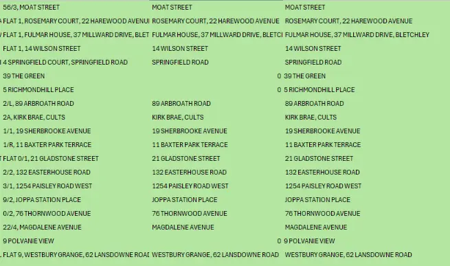
After applying the formulae leading to the separation of the particular address components, we will eventually have some records throwing errors, which by applying the condition for the IFERROR function will remain empty or show 0 or anything else. In a case such as this, we would need another column with the formula like this:
=IF(B7=0,C7,B7)
which will bring the records from two columns into one as shown below (Pic. 1).
5. Our next step is the extraction of the street number. It’s quite trivial in the case when the number was in the same separation along with the street name. Then we can apply the formula, which will extract the number from our string:
=IFERROR(TEXTJOIN("",TRUE,IFERROR((MID(D9,ROW(INDIRECT("1:"&LEN(D9))),1)*1),"")),"0")
On the other hand, we can use the FILTERXML function, which will extract everything, which is placed before the space occurring after the last number. Make sure, that your address string has been deprived of the postcode before it.
=IFERROR(LEFT(E9, SEARCH(FILTERXML("<t><s>" & SUBSTITUTE(E9, " ", "</s><s>") & "</s></t>", "//s[number()=number()]"), E9) + LEN(FILTERXML("<t><s>" & SUBSTITUTE(E9, " ", "</s><s>") & "</s></t>", "//s[number()=number()]")) - 1),0)
The first function will give us the street number, whereas the second one should include everything down to the street name like this:
FLAT 1, ROSEMARY COURT, 22
which gives us a nice way to extract the house name.
6. The house name can be obtained by the extraction of the text from the middle of our current string. The text must not include any numbers and can be obtained by the following formula:
=IFERROR(MID(AK8, FIND(",", AK8) + 1, FIND(",", AK8, FIND(",", AK8) + 1) - FIND(",", AK8) - 1),"")
but because not each of our cases includes the house number due to previous shifting towards the street name we can use our initial address string based in column A and use the ChatGPT for rendering the formula, which looks as follows:
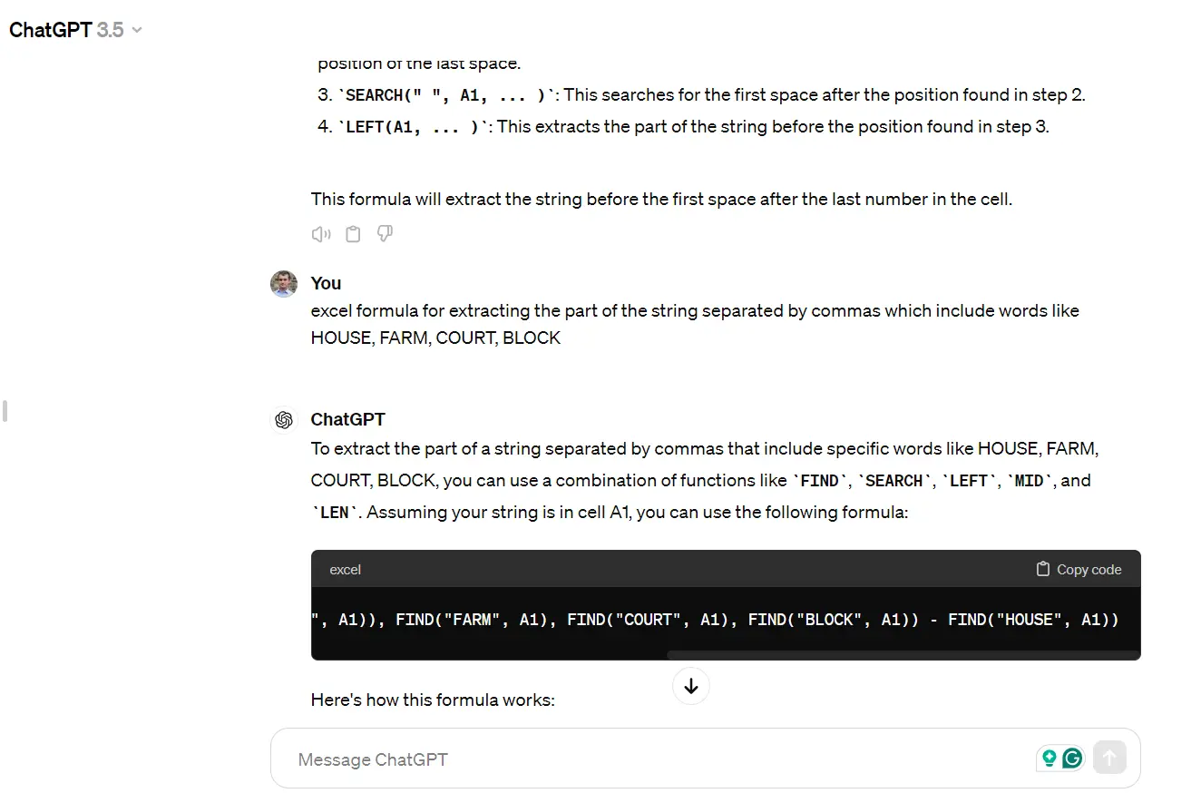
=IF(ISNUMBER(SEARCH(" HOUSE", RIGHT(MID(BC8, FIND(",", BC8) + 1, FIND(",", BC8, FIND(",", BC8) + 1) - FIND(",", BC8) - 1), LEN(MID(BC8, FIND(",", BC8) + 1, FIND(",", BC8, FIND(",", BC8) + 1) - FIND(",",BC8) - 1))))),
MID(BC8, FIND(",", BC8) + 1, FIND(",", BC8, FIND(",", BC8) + 1) - FIND(",", BC8) - 1),
IF(ISNUMBER(SEARCH(" COURT", RIGHT(MID(BC8, FIND(",", BC8) + 1, FIND(",",BC8, FIND(",", BC8) + 1) - FIND(",", BC8) - 1), LEN(MID(BC8, FIND(",", BC8) + 1, FIND(",", BC8, FIND(",", BC8) + 1) - FIND(",", BC8) - 1))))),
MID(BC8, FIND(",", BC8) + 1, FIND(",", BC8, FIND(",", BC8) + 1) - FIND(",", BC8) - 1),
IF(ISNUMBER(SEARCH(" FARM", RIGHT(MID(A8, FIND(",", A8) + 1, FIND(",", A8, FIND(",", A8) + 1) - FIND(",", A8) - 1), LEN(MID(A8, FIND(",", A8) + 1, FIND(",", A8, FIND(",", A8) + 1) - FIND(",", A8) - 1))))),
MID(A8, FIND(",", A8) + 1, FIND(",", A8, FIND(",", A8) + 1) - FIND(",", A8) - 1),
IF(ISNUMBER(SEARCH(" BLOCK", RIGHT(MID(A8, FIND(",", A8) + 1, FIND(",", A8, FIND(",", A8) + 1) - FIND(",", A8) - 1), LEN(MID(A8, FIND(",", A8) + 1, FIND(",", A8, FIND(",", A8) + 1) - FIND(",", A8) - 1))))),
MID(A8, FIND(",", A8) + 1, FIND(",", A8, FIND(",", A8) + 1) - FIND(",", A8) - 1),
""
)
)
)
)
Next, it’s vital to combine 2 columns by using the IF statement, analogical to the one shown above.
7. Extraction of the house number is the very last step and might be tricky, as some house numbers are mixed with street numbers. The most reasonable solution is the extraction of the number falling beyond the “/” character, where we can use for example the TEXTAFTER function. It’s got to get rid of the “FLAT” text too. If for example, the street number coincides with the flat number, we can try to compare it with the column, where the street number was already extracted. If the Excel formula finds the similarity, we can exclude the number and provide only the content falling beyond the “/” character. If not, we can use the whole number division.
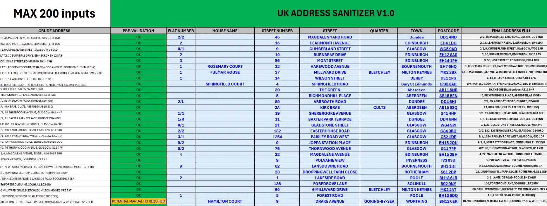
8. Pre-validation of the address is needed in case any of our formulae can guarantee the full address sanitization. Some situations might not be avoidable like swapping between the street number or house number and vice versa. In a case such as this, it’s good to inform the user, that this particular address will require manual fixing. The margin of error is estimated to be at about 5%. We need the formula, which will at some point compare our initial address with the final address received after sanitization. One of the formulas can lead us to check if the “–” symbol occurs. Another one can tell us about the occurrence of the street name in the correct place. By combining them we can get the desired result.
9. This is only a summary of the work, which falls under the first stage of tool preparation. The second one is the simplest – styling. Apart from providing the background, fonts, and borders for the cells and columns we would need conditional formatting for the validation column. Our document should look very nice at this stage (Pic. 3).
10. When styling is complete, we can equip our document with the geocoding tool. I used the Bing one for this purpose, which features good detail and it’s for free. You can spend 10K on geocoding records. The geocoding template can be attached to our worksheet easily, which is explained in detail here. After that, your Excel worksheet will be able to geocode the sanitized addresses straight away.
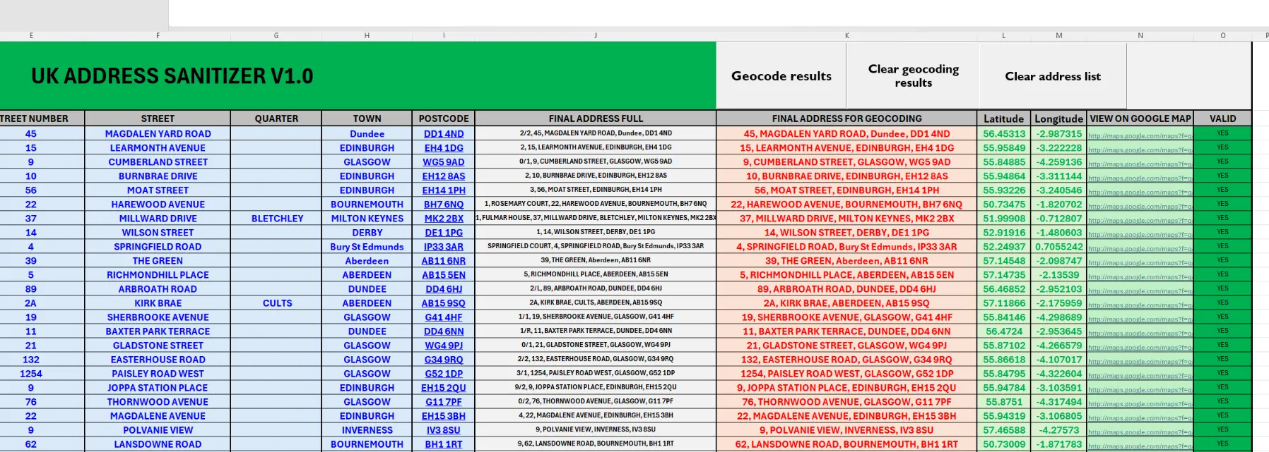
Our tool must be flexible, therefore we will need additional buttons for it. One button will refer to the macro making the geocoding for us, another two will be used for clearing the geocoding results or clearing the address list by applying the simple ClearContents for the selected range in VBA Excel.
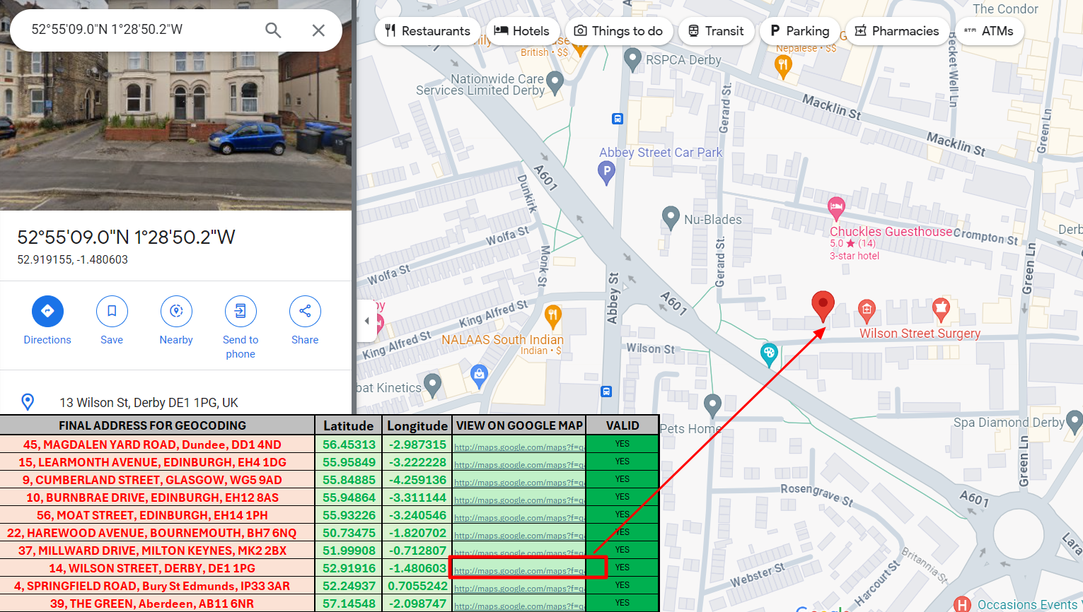
Another cool advantage of the tool is an option for visibility of our address on Google Maps (Pic. 5) by applying the HYPERLINK function to our column.
This tool can be applied to various types of UK addresses, which are stored in Excel. This is the Excel-based continuation of the thread mentioned at the beginning. It’s also a perfect example of incorporating the Bing geocoding API into your workbook.
Mariusz Krukar
Links:
- https://www.ablebits.com/office-addins-blog/excel-right-function/
- https://www.ablebits.com/office-addins-blog/excel-mid-function/
- https://exceljet.net/functions/isnumber-function
- https://www.sturppy.com/formulas/filterxml-excel-formula
- https://exceljet.net/functions/textafter-function
- https://exceljet.net/functions/hyperlink-function
Youtube: