Good way to sanitizing a bulk address list, part 1 – Excel & VBA
When you work with any Excel data, probably you experienced sometimes, that the spreadsheet input looks messy. I personally deal with the address data predominantly, which you could notice by reading my previous articles about geocoding and reverse geocoding. What is the most fun here, even the reverse geocoding results can bring confusion to our spreadsheet In other words, the address we have got includes the parts not needed at all, such as the district name, county name, country, and so on. Obviously, that depends upon your point of view, if your working area exceeds one country, then you might need the country name in your address string, and so forth. I am frankly aimed at the basic and clear address string, which can be widely used i.e. for opening some map platform roughly in place. On the other hand, this article leads also to sanitizing the bulk list of addresses, which includes a lot of repeatable sites. We always have the situation, when some block of flat is allocated for a certain postcode. However, in my opinion, there is no space for redundancy, listing all the premises one by one from this block of flat, unless we need to do so (we have allocated for example UPRN). We can compact all these repeatable addresses into one under one postcode, which might be definitely helpful for further geocoding, which as we know is usually limited.
Some approach to the clearing up of one address string has been done in this article, where I showed how to launch Google Maps straight from Excel. Today I am going to back to it for a while, although the main goal of this writing is tidying up a bulk address list with its final preparation to download as a .csv file.
- SINGLE ADDRESS STRING
First of all, let’s have a look at what can we do with a single address string below. All the elements are predominantly comma-separated, which facilitates our operations.
| 1 Willow Court, 1192 Christchurch Road, Bournemouth, BH7 6EG |
Now I have listed all the things below, which can be done with this address string. Obviously, some of them will be very similar to my previous approach.
A. TRIM() function – removes all unnecessary spaces in our string. I mean here is the situation, when our address string starts not from the very first character, but from the second or even third for example. At first glance, we won’t spot it at all. The problem becomes visible when we use some formula for string extractions, which result can make us disappointed.
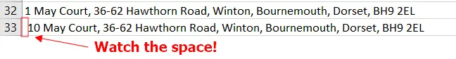
Pic. 1 Typical situation, where the address string commences with space.
Assuming, that your initial address string is in cell A1, you can use the following formula:
=TRIM(A1)
B. SUBSTITUTE() function – very useful, if we want to remove text by matching. In our case, we can do it so, since our address string is far too long and we are in the position to consider, which elements roughly are needed. We don’t need for sure the county here. We can easily get rid of it by using the expression below:
=SUBSTITUTE(A1,”Dorset, “,””)
We should remember about a whole piece, including the comma too. Otherwise, the text will be removed and the comma remained, making some of our formulas not useful. We are removing both the substring as well as the comma and space related to it. That’s why the second quote is a bit further from the comma.
Sometimes, we have a situation, where two or more substrings are unwanted in our address, like below.
| 1 Willow Court, 1192 Christchurch Road, Winton, Bournemouth, Dorset, BH7 6EG |
In this event we should nest the SUBSTITUTE() function in another SUBSTITUTE() function, like here:
=SUBSTITUTE(SUBSTITUTE(A1,”Winton, “,””),”Dorset, “,””)
making finally our problem solved.
Don’t forget, that you can both include more SUBSTITUTE() functions, by nesting them in each other as per in the example provided and also combine them with the aforementioned TRIM() function, making our spreadsheet smarter by keeping everything in one column. Our final formula should look like then:
=TRIM(SUBSTITUTE(SUBSTITUTE(A1,”Winton, “,””),”Dorset, “,””))
where everything, which subtle the TRIM() function is in the brackets likewise the cell above. Our final address will be shorter and tidy.
| 1 Willow Court, 1192 Christchurch Road, Bournemouth, BH7 6EG |
Now we have only this stuff, which potentially is needed: the flat number with the own residential building name, the street with number, city, and postcode. Let’s have a look at how can we get the data from our address.
I. LAST WORD EXTRACTION – this is important, especially when we want to extract the postcode only, falling usually as the last part of our string. The thing is straightforward, as the postcode part lies usually after the last comma. The formula below will leave exactly the last substring.
=TRIM(RIGHT(SUBSTITUTE(A1,“,”,REPT(” “,100)),100))
As a result, we should get:
| BH7 6EG |
which is roughly the postcode of our address listed above.
Remember, that the formula above can be also used for extracting the last word in our string. It will be separated not by the last comma, but by the last space.
=TRIM(RIGHT(SUBSTITUTE(A1,” “,REPT(” “,100)),100))
Instead of a comma, placed between the quotes (marked red), we should leave the space blank. The tool will recognize it as space. Remember about this empty space. If you leave the quotes next to each other, the substring won’t be executed. A full explanation of how this formula works, you can find here.
There is another method of extracting the string from the end, although it’s fixed. It means, that the same amount of symbols will be returned regardless of the length of the last substring and the comma location. Strictly not recommended, when your last word or substring has a variable length. In the UK case, when we extract the postcode, the issue seems to be straight. The total number of characters including most of the UK postcodes is 7, including the one space between. The formula will look like the below:
=RIGHT(A1,7)
bringing exactly the same result as above.
Sometimes, the UK postcode can include 8 characters like this one:
| MK10 7DX |
In this case, we can use the following formula:
=TRIM(RIGHT(A1,8))
II. EXTRACT TWO LAST WORDS FROM THE STRING – also a useful formula, however, if we consider the spaces only, the result will be exactly the same as above, giving only the UK postcode.
=MID(A1,FIND(“@”,SUBSTITUTE(A1,” “,”@”,LEN(A1)-LEN(SUBSTITUTE(A1,” “,””))-1))+1,100)
| BH7 6EG |
Again, if you take a look at the spaces between the quotes, which are marked red. You can put there some symbol, which occurs in your string (preferably the comma or other). It will change things…
=MID(A1,FIND(“@”,SUBSTITUTE(A1,“,”,”@”,LEN(A1)-LEN(SUBSTITUTE(A1,“,”,””))-1))+1,100)
| Bournemouth, BH7 6EG |
…giving us the substrings before and after the last comma (everything after the preultimate comma). Watch the space here. It’s better to include a whole formula in the TRIM() function as per below.
=TRIM(MID(A1,FIND(“@”,SUBSTITUTE(A1,”,”,”@”,LEN(A1)-LEN(SUBSTITUTE(A1,”,”,””))-1))+1,100))
Alternatively, we can use a different formula for both approaches, which is displayed below.
=TRIM(RIGHT(SUBSTITUTE(A1,” “,REPT(” “,60)),120)).
| BH7 6EG |
=TRIM(RIGHT(SUBSTITUTE(A1,“,”,REPT(” “,60)),120))
| Bournemouth, BH7 6EG |
The difference between the previous approach and this one lies in the comma, which has been removed from here.
III. EXTRACT LAST 3 OR MORE TEXTS FROM THE STRING – Sometimes we need to do so. In this case, the following formula will be applicable.
=RIGHT(A1,LEN(A1)-FIND(“~”,SUBSTITUTE(A1,” “,”~”,4)))
The result below looks as follows:
| Christchurch Road, Bournemouth, BH7 6EG |
Important here is to understand how the aforementioned formula works. The formula includes the RIGHT() function, which nests the expression used for extraction of the substrings from the left (which will be discussed later). I have marked red two elements, where the first means the symbol, to which we want to refer in our string (empty space, comma, or other), and the second includes the number of this symbol in the string, ordering it from the beginning as shown in the image below (Pic. 2).
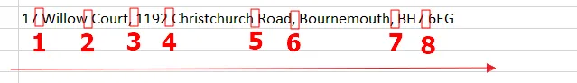
Pic. 2 The order of empty spaces in the considering string.
All considered symbols or empty spaces are ordered from the left to the right (from the beginning of the string to the end). So if we put for example 4, as we did in our formula, we should get everything after the 4th space, and so on. If we place a comma between the quotes, then we should consider the total amount of commas present in our string. If the number in the formula exceeds the number of symbols available in the string, then the #VALUE error will be thrown.
IV. EXTRACT TEXT AFTER THE FIRST COMMA – quite similar to the situation discussed above. If we don’t need the block name and number of premises in our address, we can go with the formula and result below:
=MID(A1,FIND(“,”,A1)+1,LEN(A1))
| 1192 Christchurch Road, Bournemouth, BH7 6EG |
by removing the comma from the quotes, we are getting everything after the first space. In this event, it’s the full address without the premise number.
=MID(A1,FIND(” ” ,A1)+1,LEN(A1))
| Willow Court, 1192 Christchurch Road, Bournemouth, BH7 6EG |
The alternative below works exactly the same:
=MID(A1,SEARCH(“,”,A1)+1,LEN(A1))
=MID(A1,SEARCH(” “,A1)+1,LEN(A1))
=RIGHT(A1,LEN(A1)-FIND(“,”,A1))
=RIGHT(A1,LEN(A1)-FIND(” “,A1))
by keeping the “+1“, we are preventing the new string from the comma occurrence at the very beginning.
IV. EXTRACT TEXT BEFORE THE LAST COMMA – This is needed when we want to have an address without the postcode. It represents quite the opposite situation to the point I considered above. In this event, we need some addresses, without the postcode. We have effectively 2 approaches to this situation. The first one will extract always everything before the last comma, regardless of the total number of commas in our whole string:
=MID(A1,1,FIND(“@”,SUBSTITUTE(A1,“,”,”@”,LEN(A1)-LEN(SUBSTITUTE(A1,“,”,””)))))
giving in our case the following result:
| 1 Willow Court, 1192 Christchurch Road, Bournemouth, BH7 6EG |
which can be a bit smarter, when we remove the last existing comma behind “Bournemouth” by adding “-1” to our formula like below.
=MID(A1,1,FIND(“@”,SUBSTITUTE(A1,“,”,”@”,LEN(A1)-LEN(SUBSTITUTE(A1,“,”,””))))-1)
I have marked some stuff red intentionally, which you can play with by adding the character, which occurs in your address string or simply leaving the empty space between these quotes. In this event, the formula will return everything without the last sentence, separated by the last space in our string:
=MID(A1,1,FIND(“@”,SUBSTITUTE(A1,” “,“@”,LEN(A1)-LEN(SUBSTITUTE(A1,” “,””))))-1)
| 1 Willow Court, 1192 Christchurch Road, Bournemouth, BH7 |
but we certainly don’t want to have only one piece of postcode in this case. Anyhow it’s good to know about the way like this. This formula is also considered later, as we have a bit more combinations available here.
Another way to sort the issue is a bit simpler, although we should know roughly how many commas occur in our address string. Taking into account, that we have them 3, the formula should look like the below:
=LEFT(A1,FIND(“~”,SUBSTITUTE(A1,“,”,”~”,3)))
and our address, instead of the full string:
| 1 Willow Court, 1192 Christchurch Road, Bournemouth, BH7 6EG |
should be reduced by the postcode:
| 1 Willow Court, 1192 Christchurch Road, Bournemouth, |
with obviously an option of removing the third comma at the very end, by adding “-1” to our formula. Whereby we should put the “-1” just before the last bracket, related to our LEFT() function.
=LEFT(A1,FIND(“~”,SUBSTITUTE(A1,“,”,”~”,3))-1)
Again, the stuff included in red, between the quotes gives us an opportunity to swiftly alter the formula, by changing the symbol or giving the empty space there. The result will be analogous. Another formula can be like this:
=LEFT(A1, FIND(“^”,SUBSTITUTE(A1, “,”, “^”,3)&”^”))
where we are defining before which comma our substring should be extracted.
In the UK postcode situation, knowing that they’re pretty much fixed in their lengths, we can also use this simple formula:
=LEFT(A1,LEN(A1)-9)
or
=TRIM(LEFT(A1,LEN(A1)-10))
by removing the last 9 or 10 characters from our string (7 or 8 characters including the postcode, 1 space, and the last comma – 7+1+1).
| 1 Willow Court, 1192 Christchurch Road, Bournemouth |
V. EXTRACT MORE THAN 2 FIRST SUBSTRINGS/EXTRACT WORDS BEFORE 2ND COMMA – Needed sometimes when we want to keep for instance the house number, house name, and street address only. In this case, we should take a look at how they are separated by commas or other symbols. If we have made sure about this, we can go ahead with the last described formula:
=LEFT(A1,FIND(“~”,SUBSTITUTE(A1,“,”,”~”,2))-1)
extracting only the things I mentioned above.
| 1 Willow Court, 1192 Christchurch Road |
The same result we are getting from the following formula:
=IF((LEN(A1)-LEN(SUBSTITUTE(A1,“,”,””)))<2, A1, LEFT(A1,FIND(“,”,A1, FIND(“,”,A1)+1)-1))
where we should remember the “+1” character.
Another formula brings exactly the same result:
=LEFT(A1, FIND(“,”, A1, FIND(“,”, A1)+1 ) – 1)
but removing any of the red commas will result in downgrading our string to the text before the 1st comma occurs.
The last way:
=TRIM(LEFT(SUBSTITUTE(A1,“,”,REPT(” “,100)),200))
gives the same result but with no comma at all.
| 1 Willow Court 1192 Christchurch Road |
When the marked comma is removed from the quotes, the tool will extract the first two words from our string only.
There is also another formula, that can allow us to extract a various number of strings, however, we must make sure regarding our address string, and define what we want to have extracted from it.
=LEFT(TRIM(A1),FIND(“^”,SUBSTITUTE(TRIM(A1)&” “,” “,”^”,6))-2)
| 1 Willow Court, 1192 Christchurch Road |
In this case, the number 6 means roughly the 6 single words in our string from the very beginning, and another “-2” indicates where the substring stops (before the 7th space and comma before). Make sure, that you have the comma at the end of the substring you want to get. Otherwise, I would advise you to put “-1” instead.
The last solution can be too time-consuming, although it’s good to know about it. The result is exactly the same as above. The formula looks as follows:
=IF((LEN(A1)-LEN(SUBSTITUTE(A1,” “,””)))<3,A1,LEFT(A1,FIND(” “,A1,FIND(” “,A1,FIND(” “,A1,FIND(” “,A1,FIND(” “,A1, FIND(” “,A1)+1)+1)+1)+1)+1)-2))
where each FIND() function corresponds to the single word in our string. By adding the comma in the brackets, we can expand our substring by 1 word beyond this comma:
=IF((LEN(A1)-LEN(SUBSTITUTE(A1,” “,””)))<3,A1,LEFT(A1,FIND(” “,A1,FIND(” “,A1,FIND(” “,A1,FIND(” “,A1,FIND(” “,A1, FIND(“,”,A1)+1)+1)+1)+1)+1)-2))
| 1 Willow Court, 1192 Christchurch Road, Bournemouth |
but it works for a fixed number of words in the string. If at some point our address changes i.e. the house name will be comprised of three words, the substring won’t reach the city. Bear that in mind.
VI. GET FIRST TWO WORDS/EXTRACT PART BEFORE 1ST COMMA – a quite often useful operation. In the address string, we typically get the house name and its number or the street name with number, when we have a single dwelling unit. In this case, we have quite a few ways to sort it out. Following the formula above, we need to change only the “2” into “1“, as this number defines the comma order in our string. It does the same regarding space also (Pic. 2).
=LEFT(A1,FIND(“~”,SUBSTITUTE(A1,“,”,”~”,1))-1)
By keeping all the things described above with this smallish change, we can get finally:
| 1 Willow Court |
as well as after this formula:
=LEFT(A1,FIND(“~”,SUBSTITUTE(A1,” “,”~”,3))-2)
where I have removed the comma, changed the number to 3 (the 3rd space from the beginning), and added -2 characters from the end in order to remove the unwanted comma.
Another approach is using the previous formula above, in which we could extract everything before the last comma. Now, we must change some things…
instead of
=MID(A1,1,FIND(“@”,SUBSTITUTE(A1,”,”,“@”,LEN(A1)-LEN(SUBSTITUTE(A1,”,”,””))))-1)
we should write
=MID(A1,1,FIND(“,”,SUBSTITUTE(A1,”,”,“,”,LEN(A1)-LEN(SUBSTITUTE(A1,”,”,””))))-1)
In place of “@” which allowed us to skip to the last comma, we should put “,“. Then an extract substring will be restricted by the first comma. It works analogically in terms of the space but I will back to it later.
The third approach is the following formula:
=IF((LEN(A1)-LEN(SUBSTITUTE(A1,” “,””)))<2, A1, LEFT(A1,FIND(“,”,A1, FIND(” “,A1)+1)-1))
or just another way around:
=IF((LEN(A1)-LEN(SUBSTITUTE(A1,“,”,””)))<2, A1, LEFT(A1,FIND(“,”,A1, FIND(“,”,A1))-1))
where the smartest way is simply to remove the “+1” from the formula.
Another formula also discussed above is:
=TRIM(LEFT(SUBSTITUTE(A1,” “,REPT(” “,100)),200))
however, we can use also others, like:
=LEFT(A1, FIND(“,”, A1, FIND(” “, A1) + 1) – 1)
The last approach can look like this:
=IFERROR(LEFT(A1,FIND(“,”,A1)-1), A1)
VIII. GET FIRST WORD – common situation, however not as useful in terms of address as it could be. In our situation, we can get the street or flat number only, whatever comes at the beginning of our address string. Moreover, we cannot rely on these numbers, because in fact, sometimes the flats have numeration like 12A, 12B, 13A, and so forth. The presence of the letter along with a number (unless it’s separated by the space, which happens very rarely) excludes this data from further processing unless we provide another function able to remove an unwanted character.
The basic formula, which allows us to extract the very first word from our address string looks as follows:
=LEFT(A1 , SEARCH(” “,A1 ))
where between the quotes must be the space, defining the very first space occurrence in our string. Finally, we are getting the house or street number whatever comes as a first in our address.
| 1 |
Exactly the same result we can get when applying other formulas:
=MID(A1,1,FIND(” “,SUBSTITUTE(A1,”,”,” “,LEN(A1)-LEN(SUBSTITUTE(A1,”,”,””))))-1)
=LEFT(A1, FIND(“^”,SUBSTITUTE(A1, ” “, “^”,1)&”^”))
=LEFT(A1,FIND(“~”,SUBSTITUTE(A1,” “,”~”,1))-1)
=TRIM(LEFT(SUBSTITUTE(A1,” “,REPT(” “,100)),100))
=LEFT(A1,FIND(” “,A1, FIND(” “,A1))-1)
=LEFT(TRIM(A1),FIND(“^”,SUBSTITUTE(TRIM(A1)&” “,” “,”^”,1))-1)
IX. EXTRACT WORD FROM THE MIDDLE OF THE STRING – Very useful from our point of view, especially, when we need to extract for example the name of a town from our whole address string. The most convenient way for it is using the FILTERXML() function, which can look as below:
=FILTERXML(“<t><s>”&SUBSTITUTE(F1,”, “,”</s><s>”)&”</s></t>”,”//s[position()=last()-1]”)
the formula is targeted at the last position of our string. However, by adding “-1” we are moving one section backward, extracting it. So if our initial address looks as below:
| 1 Willow Court, 1192 Christchurch Road, Bournemouth, BH7 6EG |
we should be able to extract the name of our city, which falls at the penultimate substring defined by commas.
| Bournemouth |
Another way is more complicated with the following formula:
=MID(A1, SEARCH(“,”,A1) + 1, SEARCH(“,”,A1,SEARCH(“,”,A1)+1) – SEARCH(“,”,A1)-1)
although following the basic MID() function understanding, we can only get the stuff after the first symbol is observed. In our case, after the first comma then.
| 1192 Christchurch Road |
If we want to get the name of our city, involving another cell will be required.
X. EXTRACT TWO WORDS FROM THE MIDDLE OF THE STRING – This is possible with the formulas above when they aren’t comma-separated from each other. In the different cases, we can use very similar formulas, but expand a little bit, as shown below:
=TEXTJOIN(“, “,,FILTERXML(“<t><s>”&SUBSTITUTE(A1,”, “,”</s><s>”)&”</s></t>”,”//s[position()=2 or position() =3]”))
| 1192 Christchurch Road, Bournemouth |
The FILTERXML() function can be expanded on other substrings when we change position()=last() to position()=substring_number and add also or option as per above. Unfortunately, this solution won’t bring us the result, we would expect, because the extracted stuff will occupy two cells. The result is returned to neighboring cells, which is called spilling. Spill means, that formula has resulted in multiple values, where some of them go to adjacent cells. We definitely want a whole result in one cell. For this purpose, we should embed this whole function in another one – TEXTJOIN() (Pic. 3).
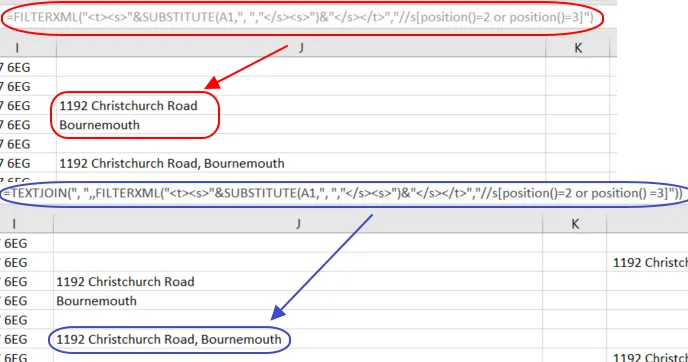
Pic. 3 The subtle difference in our result when we use the TEXTJOIN function or not.
Another solution comes from the MID() function formula discussed above. As you can see, this formula includes more than 1 SEARCH() element. If we need to expand our result, we should embed another element, where instead of:
=MID(A1, SEARCH(“,”,A1) + 1, SEARCH(“,”,A1,SEARCH(“,”,A1)+1) – SEARCH(“,”,A1)-1)
we should write:
=MID(A1, SEARCH(“,”,A1) + 1, SEARCH(“,”,A1,SEARCH(“,”,A1,SEARCH(“,”,A1)+1)+1) – SEARCH(“,”,A1)-1)
expanding a range of our extract, but still after the first symbol occurrence (in our case it’s a comma).
| 1192 Christchurch Road, Bournemouth |
After these 10 major ways of manipulation with address string, I would like to add another one as the outreach.
A. REMOVE SPECIFIED SYMBOL FROM THE STRING – In our case, it’s the comma. Because our address string includes about 3 or 4 commas, we can remove one of them. Regarding the MID() function described above it can be useful. Let’s have a look again at how our address initially looked like:
| 1 Willow Court, 1192 Christchurch Road, Bournemouth, BH7 6EG |
with all the commas marked red. If, for example, we want to remove the last comma, we should all count all the commas from the very beginning and likewise state an analog image above (Pic. 2). Then implement the SUBSTITUTE() function as per below:
=SUBSTITUTE(A1,”,”,” “,3)
where we are removing the 3rd comma (last in our order). Thereafter the address string has changed slightly.
| 1 Willow Court, 1192 Christchurch Road, Bournemouth BH7 6EG |
2. BATCH ADDRESS SANITIZING
Batch sanitizing our address list can be quite easy when we know how to apply the formulas described above. It obviously depends on what we want to have as the final result. Assuming, that we have the correct address string like the one considered before, we should take into account, especially the TRIM() and SUBSTITUTE() functions.
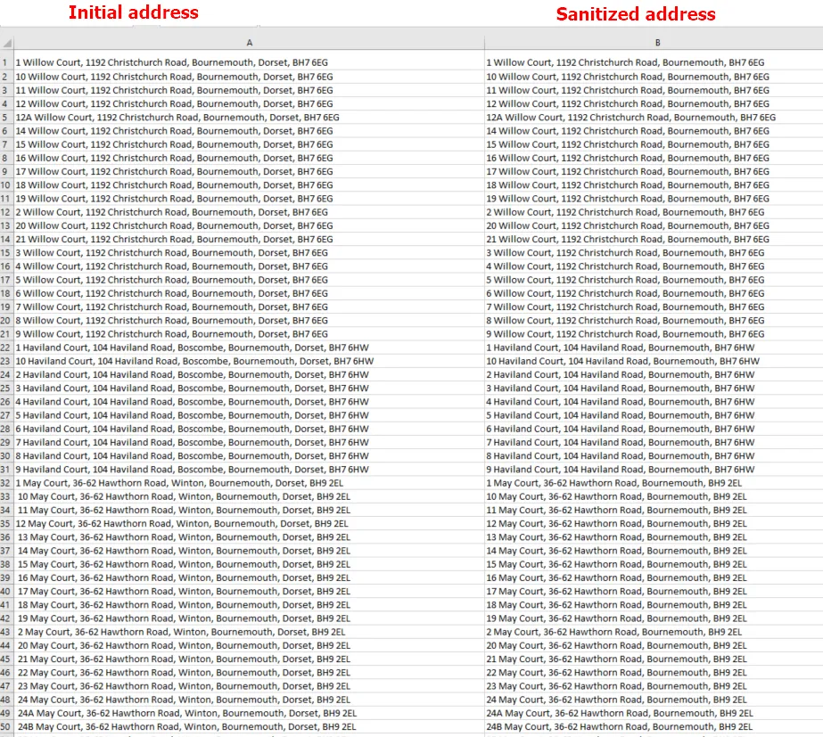
Pic. 4 The TRIM() and SUBSTITUTE () functions are able to sanitize our address strings quickly.
The example formula, which has been used here is:
=TRIM(SUBSTITUTE(SUBSTITUTE(A26,”Boscombe, “,””),”Dorset, “,””))
and we can admit, that our job looks really good.
Another problem, which should be solved here is the address redundancy. Basically, every single address corresponds to the unique UPRN number (as we are considering the UK address). In turn, there are at least several exactly the same addresses allocated to one place. The difference lies in the number of the premises only. Our task here is to compress all these repeatable addresses into one. For this purpose, I could use the following formulas:
A. EXTRACTING THE HOUSE NUMBER AND HOUSE NAME ONLY (OPTIONALLY TO THE COLUMN C)
=LEFT(B1,FIND(“~”,SUBSTITUTE(B1,”,”,”~”,1))-1)
B. EXTRACTING ONLY THE HOUSE NUMBER (OPTIONALLY TO THE COLUMN D) – here the issue can be tricky, as discussed previously. We cannot rely on all the formulas used widely for getting the first word from our string. Because, if we have the address like this:
| 12A Willow Court |
we will get:
| 12A |
and it won’t work for our further purposes.
We should implement another formula:
=LEFT(C1,SUM(LEN(C1)-LEN(SUBSTITUTE(C1,{“0″,”1″,”2″,”3″,”4″,”5″,”6″,”7″,”8″,”9″},””))))*1
which will extract only the number string for us. However, because this string is still treated as the text, I would advise putting “*1” at the very end, making the result numerical.
| 12 |
Alternatively, we can use some of the functions described above and embed them into the SUBSTITUTE() function, like below:
=SUBSTITUTE(SUBSTITUTE(LEFT(A1, SEARCH(” “,C1 )),”A”,””),”B”,””)*1
assuming, that our flat numbers will be A or B only.
C. EXTRACTING THE HOUSE NAME ONLY (OPTIONALLY TO THE COLUMN E) – Another part, we definitely need here. If then our house name with number has been extracted to column C, and the number only to column D, we can now use column E.
With this formula for example:
=RIGHT(C1,LEN(C1)-FIND(“~”,SUBSTITUTE(C1,” “,”~”,1)))
we can get the house name.
| Willow Court |
D. REMOVE THE HOUSE NUMBER AND HOUSE NAME (OPTIONALLY COLUMN F) – this is the thing, we can do optionally, by using this formula:
=RIGHT(B1,LEN(B1)-FIND(“~”,SUBSTITUTE(B1,”,”,”~”,1)))
and extract what we want from the column B as per below:
| 1192 Christchurch Road, Bournemouth, BH7 6EG |
leaving the address without the home name and premise number, which belongs to it.
E. EXTRACTING THE TOWN/CITY NAME (OPTIONALLY COLUMN G) – we can potentially need it, so it’s a good moment to use one of the formulas extracting the substring from the middle of the main string:
=FILTERXML(“<t><s>”&SUBSTITUTE(F1,”, “,”</s><s>”)&”</s></t>”,”//s[position()=last()-1]”)
| Bournemouth |
F. REMOVING POSTCODE (OPTIONALLY COLUMN H) – we can desire the address and postcode separately, so it’s good to split them just in case. Since column F has been considered as the street address without the house number and name, we can get split it easily. First of all, we will remove the postcode by the following formula:
=LEFT(F1,FIND(“~”,SUBSTITUTE(F1,”,”,”~”,2))-1)
receiving finally the street address only.
| 1192 Christchurch Road, Bournemouth |
G. EXTRACTING POSTCODE IN THE SEPARATE COLUMN (OPTIONALLY I) – the second part of our operation. The postcode can be extracted twofold, as the stuff after the last comma or the last two words in the string. Because I am dealing with the UK postcode, pretty much fixed in its length, I can simply use the following formula:
=RIGHT(A1,7)
or
=TRIM(RIGHT(A1,8))
which can be risky in other situations. I can extract the postcode from columns A, B, or F.
H. THE LOWEST AND THE HIGHEST NUMBER – Very useful in our purpose. Because we have a set of repeatable addresses, which finally represent some range. We should definitely determine the lowest and the highest house number from this address range. Instead of searching it manually throughout 20 rows on average, we can simply use the MIN() and MAX() formulas.
=MIN(range)
=MAX(range)
I. FINDING THE CURRENT ROW – also a useful function, which we will need here. It’s defined by the
=ROW()
function, which should return us to the current row for the active cell we working on.
J. CALCULATING A TOTAL NUMBER OF RECORDS – It should be done at the very beginning fairly. We can get to know straight away how many single address inputs we are dealing with. This formula will sort it out for us:
=ROW(OFFSET(A1,COUNTA(A:A)-1,0))
whereas we have to take into account the very first column, where all our messy addresses are stored. In my case, the result is shown below.
| 1080 |
By knowing the total amount of my records I am able to define the full range of rows I am going to work on.
K. COUNTING CELLS WITH THE SPECIFIC TEXT – In our case, we can figure out how many postcodes fall under the 1 address fairly. As considered, our messy list includes at least several of the same addresses allocated to the same location, defined by the same street number or postcode. In this case, we are going to count the total number of certain postcodes in our whole range:
=COUNTIF(I$1:I$1080,”BH7 6EG”)
We are using column I, where the postcode has been extracted, covering our whole range with 1080 records exactly.
If you have a bulk address list, this approach can be quite long. In this event, I would advise referring the COUNTIF() function to the cell, where the postcode is based. The formula would look as below:
=COUNTIF(I$1:I$1080, “”& I1)
whereas we should always remember the quotes here.
The number of flats under the BH7 6EG postcode is:
| 21 |
L. DETERMINING THE LAST ROW OF CURRENT ADDRESS GROUP/CURRENT POSTCODE – needed in order to simplify our further formulas. Since we know the number of addresses falling under one postcode, we can quickly calculate the range of rows, where the current postcode occurs (Pic. 5).
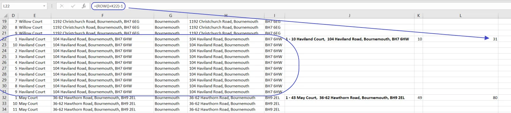
Pic. 5 Determining the last row in our current address range in Excel. Click to enlarge.
=(ROW()+K22)-1
We should always subtract 1 row, as the first one is usually the active row we are working on. Unless you start from the very top, then you don’t need to do so.
=ROW()+K1
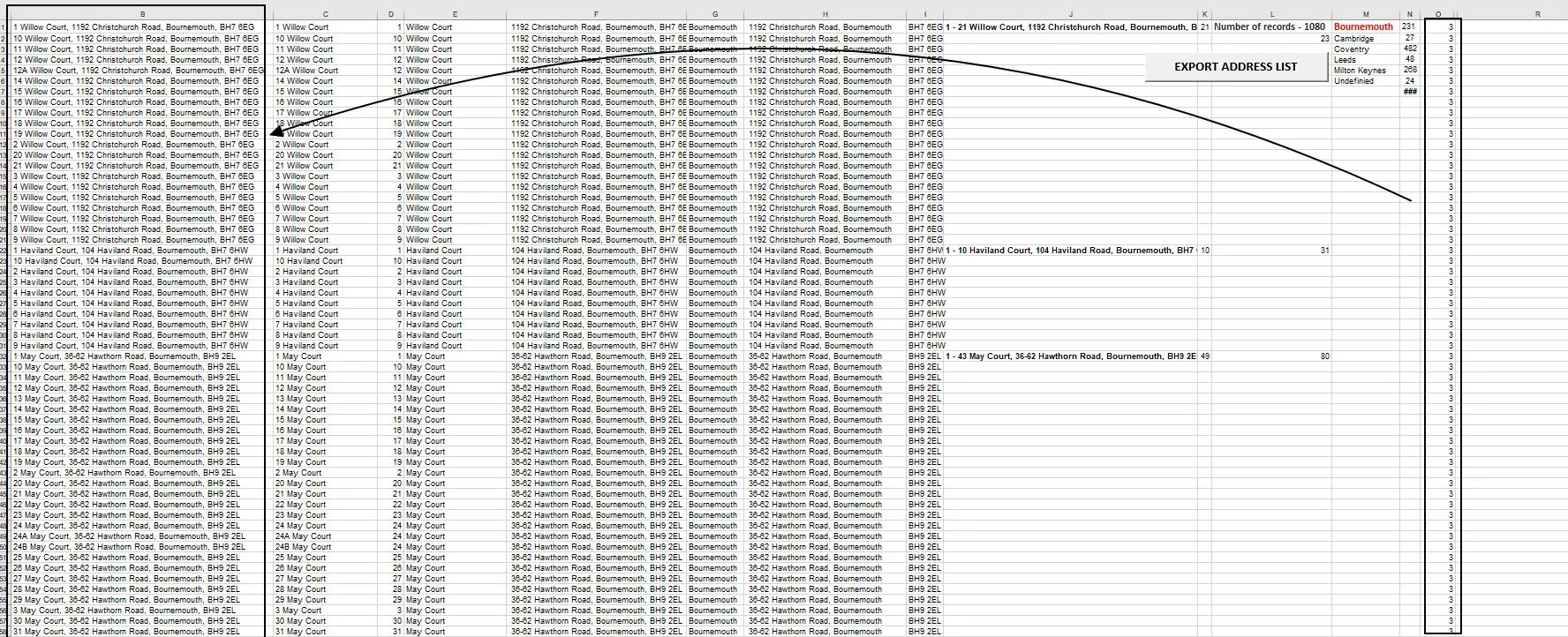
M. CONCATENATE() function – as a final step of our work. This function combines all the stuff we want and merges it into one value/string in the cell. In my case, it looks as follows:
=CONCATENATE(MIN(D1:D21),” – “,MAX(D1:D21),” “,E1,”,”,F1)
where the MIN() and MAX() functions are already included. The final range D1:D21 will be a derivative from the aforementioned ROW() function. However, you can always provide it manually, whatever is suitable for you.
I also did the CONCATENATE() function to highlight the total amount of my records:
=CONCATENATE(“Number of records – “,ROW(OFFSET(A1,COUNTA(A:A)-1,0)))
| Number of records – 1080 |
My final results are:
| 1 – 21 Willow Court, 1192 Christchurch Road, Bournemouth, BH7 6EG |
which is seemingly nothing, but as you might have noticed, instead of 21 repeatable addresses I have got one, including a whole range of property numbers allocated for this street number and postcode. It’s our final approach, although we should make the last step of our work, which includes some VBA Excel coding. Before we do that, let’s see the final image below including all steps of my work so far including all steps pointed in this section (Pic. 6).
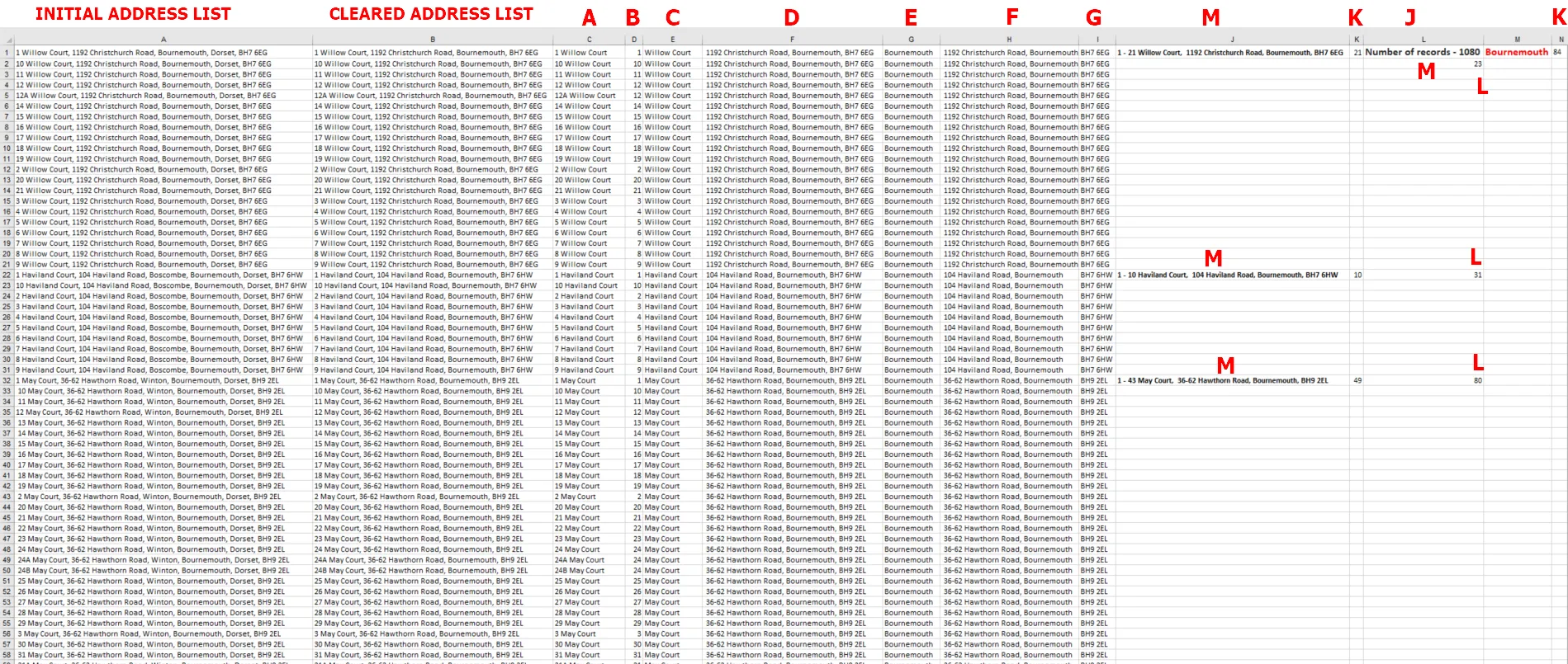
Pic. 6 All steps leading to address sanitization where: A – extracting the house number and house name; B – extracting the house number only; C – extracting the house name only; D – removing the house number and house name from the string, keeping the street address with postcode only; E – extracting the town/city name; F – removing postcode from our address; G – extracting postcode as a single string; J – calculating a total number of records; K – counting cells with the specific text; L – determining the last row of a current postcode (based on the point I not shown in the picture); M – concatenate function for the lowest and highest number values (point H not covered in the image) and all columns needed to build a new address string. Click to enlarge.
I also calculated the total number of records with the given city (Pic. 6, Col. N).
3. UNFORESEEN SITUATIONS AND ALTERNATIVE APPROACHES
Sometimes we have a situation when more than one postcode is allocated for one address, especially when the number of flats is high. In this event, we can manually clear the mismatches, which cover:
– finding the highest flat number for the given postcode
– finding the lower flat number for the next postcode allocated to the same address
– changing the formula, which extracts house number for us, by removing *1, where instead of:
=LEFT(C1,SUM(LEN(C1)-LEN(SUBSTITUTE(C1,{“0″,”1″,”2″,”3″,”4″,”5″,”6″,”7″,”8″,”9″},””))))*1
we should leave:
=LEFT(C1,SUM(LEN(C1)-LEN(SUBSTITUTE(C1,{“0″,”1″,”2″,”3″,”4″,”5″,”6″,”7″,”8″,”9″},””))))
moving our numbers into the text format, which will be clearly visible in our list, as the numbers now are placed on the opposite side of the cell (Pic. 7).
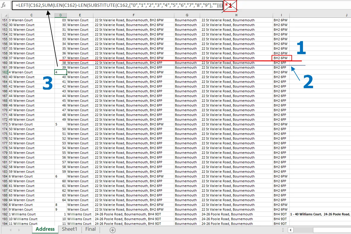
Pic. 7 Unforeseen situations, where virtually the same address is allocated to 2 postcodes. In this case, we should proceed manually by 1 – finding the highest flat number for the first postcode (define the row and apply it to the final formula); 2 – finding the lowest flat number for the second postcode and applying it to the final formula; 3 – Remove the “*1” character from the excel formula discussed. In turn, all the numbers fall on the other side of the cell and are excluded from MIN() and MAX() functions. Click to enlarge.
Obviously, I assume, that you do have not many addresses like this and you don’t want to play with another column separately.
You can also subtract the value from the MAX() function.
=CONCATENATE(MIN(D691:D722),” – “, MAX(D691:D722)-3,” “, E691,”,”,F691)
Another situation, which might happen is the “shift” of formulas. I mean, that our address has only the street number and street name without any information about the particular house. In this event, we can use the IFERROR() function in place, where the #VALUE is thrown. For example:
=IFERROR(RIGHT(C259,LEN(C259)-FIND(“~”,SUBSTITUTE(C259,” “,”~”,1))),””)
where any error is going to be replaced by an empty value (Pic. 8).
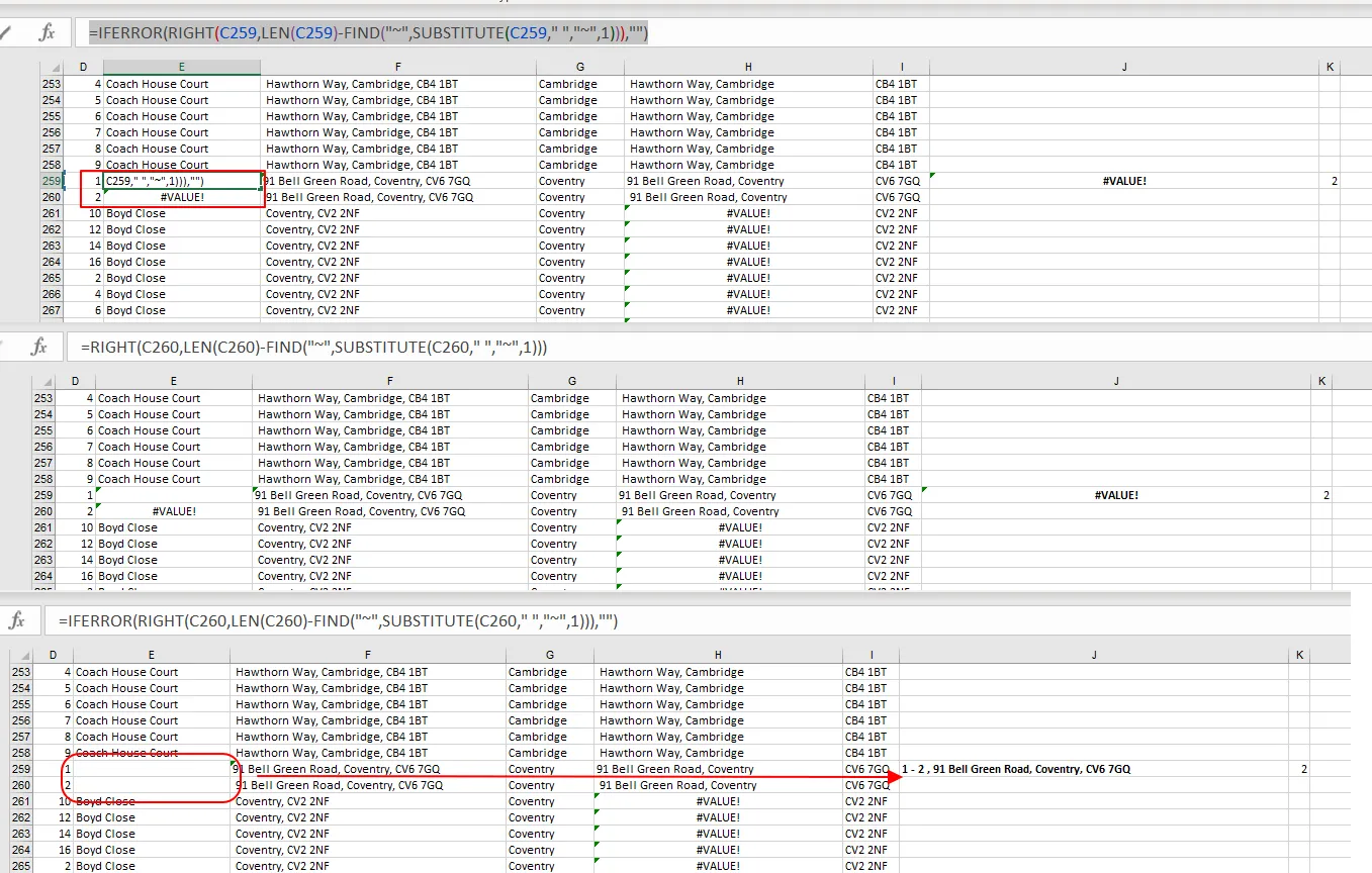
Pic. 8 Using the IFERROR() function for covering all errors in our address list caused by “shift”.
When the UK postcode is a bit longer, what happens rarely, like in Milton Keynes example:
| MK11 1NN |
=TRIM(RIGHT(A903,8))
We will get predominantly a space before the postcode in other cases, but the TRIM() function will get rid of it for us.
The last issue here is the different lengths of the addresses, as some of them don’t include the house name and number. It finally results in a lower number of commas occurring in the whole string. In our case the issue seems to be straightforward, where we have only 2 options effectively; addresses include 2 or 3 comma characters. In order to more effective sanitizing, I applied another formula to my workbook, which can calculate the number of commas for me:
=LEN(B1)-LEN(SUBSTITUTE(B1,“,”,“”))
where the comma occurrence is calculated from column B, where our new cleared address is stored (Pic. 6, 9).
Pic. 9 Calculating the number of comma occurrences in my address string. Click to enlarge.
This step can facilitate our further work a bit at the VBA coding stage, but not there certainly. If for example, you will need to split the single dwelling units allocated to the same postcode, then you can expand your CONCATENATE() function by adding the IF() statement as follows:
=IF(O1=3,CONCATENATE(MIN(D1:D21),” – “,MAX(D1:D21),” “,E1,”,”,F1),CONCATENATE(C1,”, “,F1))
where we are defining effectively 2 cases. If our address string includes 3 commas, then we know, that apart from the basic street address we have the house number too, and definitely, more than 1 number falls under the same address fairly. We will use the MIN() and MAX() functions then.
On the other hand, if our address has 2 commas (frankly other value than 3, but predominantly 2), then we can simply concatenate column C including the street name and number (after the “shift” mentioned above) and column F including solely city and postcode in this event (Pic. 10).
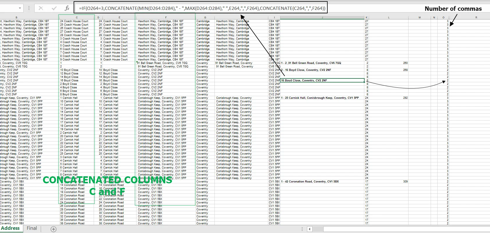
Pic. 10 Applying the IF statement for the length of our addresses. In the case shown we just need to concatenate 2 columns instead of using the MIN() and MAX() functions for the range. Click to enlarge.
In this case, when we decide to extract the single dwelling unit address regardless of the total amount of them comprising of the postcode number, I would advise providing the IF() function to COUNTIF() too. The new formula should look as follows:
=IF(O261=3,COUNTIF(I$1:I$1080, “”& I261),1)
where the function returns number 1 for us, when we encounter the address without the house number and name. Otherworldly the address includes less than 3 comas (exactly 2) in its whole string. I would advise inserting a new column, where you will keep the total number of dwellings falling under one postcode, or unless put number 1 in the row occupied by a single dwelling unit. It’s essential for our VBA code later. I will use column P for this (Pic. 11), where I will apply this simple formula:
=IF(J1<>” “,K1,””)
and rectify it to:
=IF(J1<>“”,K1,””)
because I want to have empty cells, where rows in K column values were not provided.
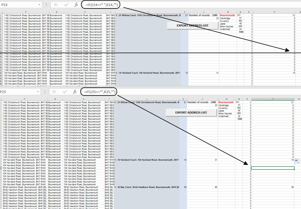
Pic. 11 Short formula accelerating our input in column P, where the total number of units is going to be based. Be aware of quotes, which have to be next to each other. Any space between them will throw 0 in our cell.
Column P is fetched by column K, where we based our COUNTIF() function for postcodes. However, if column J (where our new address occurs) is empty, then column P will be empty. By using this formula we can simply drag down and achieve the result needed for further VBA steps.
In order to accelerate your work, you can use the INDIRECT() function, which will fetch the data from the column, where you considered the last row in the given record. It’s column L (Pic. 6, L), which must be included in our MIN(), and MAX() functions now. Our formula is going to be expanded then. From the pattern above:
=IF(O1=3,CONCATENATE(MIN(D1:D21),” – “,MAX(D1:D21),” “,E1,”,”,F1),CONCATENATE(C1,”, “,F1))
we should make:
=IF(O22=3,CONCATENATE(MIN(D1:INDIRECT(“D”&L1)),” – “,MAX(D22:INDIRECT(“D”&L1)),” “,E1,”,”,F1),CONCATENATE(C1,”,”,F1))
where our L column says the last row used for the given repeatable value (our postcode).
Sometimes there are situations when we don’t have the building name, but we know, that some street numbers are comprised of the block of flats (assuming, that you have checked it before). In this case, we can use the search for the part of the string in our address, if we know roughly the street name, where this situation occurs. The formula will look like this:
=IF(ISNUMBER(SEARCH(“March”,B582)),CONCATENATE(MIN(D582:INDIRECT(“D”&L582)),” – “,MAX(D582:INDIRECT(“D”&L582)),” “,E582,”,”,F582),CONCATENATE(“,”,C582,”,”,F582))
binding all our addresses in one.
| 25-36 March Way, Coventry, CV3 2QY |
The similar formula will be applied to our postcodes:
=IF(ISNUMBER(SEARCH(“March”,B583)),(O584=3,COUNTIF(I$1:I$1080, “”& I584),1)
binding them as one from this time.
At the final stage, we have another smallish thing. Namely, if your address starts from 1-2 12 Street name, it’s highly likely, that your 1-2 number will be turned into the date when copied. To prevent this situation, we have to expand our CONCATENATE() function by adding the empty space at the very beginning. Finally, our formula will look as:
=IF(O1=3,CONCATENATE(” “,MIN(D1:INDIRECT(“D”&L1)),” – “,MAX(D1:INDIRECT(“D”&L1)),” “,E1,”,”,F1),CONCATENATE(C1,”,”,F1))
I could also place the comma at the very beginning of the shorter address. The VBA code can be simplified thanks to this. We will have a weird comma at the very beginning of our short address, but our final product is the .csv file generated by a macro, so we shouldn’t worry about it.
=IF(O1=3,CONCATENATE(” “,MIN(D1:INDIRECT(“D”&L1)),” – “,MAX(D1:INDIRECT(“D”&L1)),” “,E1,”,”,F1),CONCATENATE(“,”,C1,”,”,F1))
In the end, I would like to say: don’t be scared of a multitude of SUBSTITUTE() functions nested in each other (Pic.12). Sometimes it’s necessary.
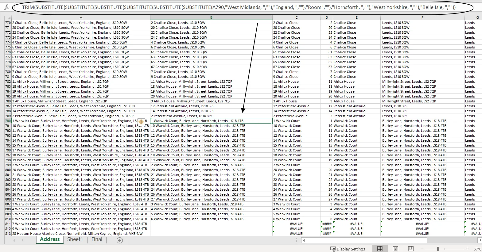
Pic. 12 An example of a multitude of SUBSTITUTE() functions nested in each other when sanitizing the addresses.
4. SANITIZED ADDRESS LIST
The last thing to do here is to prepare the final address list, with an option to straight export to a .csv file, which can be further used for interactive maps as the GeoJSON layer. We need some smart VBA code, which I am going to develop and explain a bit here. My approach is individual, and obviously, you can find another way to sort it out. The topic is open. I’ve sorted it by a few steps listed below:
– copying the data from the main sheet to another one (1),
– removing blank spaces between the new addresses (2),
– inserting new 4 columns from the left (new columns A:D, where the split address string will be stored) (3)
– splitting the data between the relevant columns (based on the comma number conditions) (4)
– removing blank spaces at the very beginning of the divided string (5)
– merging columns including street address (6)
– copying the relevant columns into the target destination, which will comprise three columns including consequently: Address, Postcode, and number of premises (7)
– giving a title for the address columns (address, postcode, number of units) (8)
– deleting unnecessary columns, (9)
– export our address list as the .csv file (10)
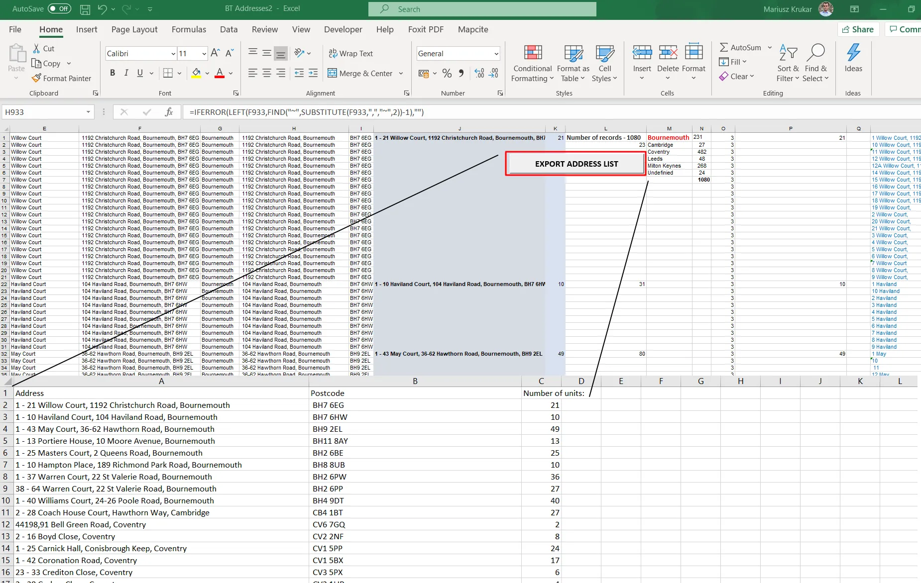
Pic. 13 New Address list in .csv file generated by button.
The VBA code describing most of the points mentioned above looks as below:
Option Explicit

Sub Exportaddress()
Dim Wksht As Worksheet, Acts As Worksheet
Dim MyArray() As String, myPath As String
Dim lRow As Long, i As Long, j As Long, c As Long

Set Wksht = ThisWorkbook.Sheets("Final")
Set Acts = ThisWorkbook.Sheets("Address")

'Copying the sanitized address and postcode from the main sheet (1)

Acts.Columns("J:K").Copy
Wksht.Columns("A:B").PasteSpecial xlPasteValues

'Removing blank spaces (2)

With Wksht.Columns("A")
.ColumnWidth = 60
.SpecialCells(xlCellTypeBlanks).EntireRow.Delete
End With

'Inserting new columns for splitting the data (3)

Wksht.Columns("A:D").Insert Shift:=xlToRight, _
CopyOrigin:=xlFormatFromLeftOrAbove

'Splitting the address data likewise "Text to columns" option, but the results come to first 4 columns (4)

With Wksht
lRow = .Range("E" & .Rows.Count).End(xlUp).Row
For i = 1 To lRow
If InStr(1, .Range("E" & i).Value, ",", vbTextCompare) Then
MyArray = Split(.Range("E" & i).Value, ",")
c = 1
For j = 0 To UBound(MyArray)
.Cells(i, c).Value = MyArray(j)
c = c + 1
Next j
End If
Next i

End With

'Removing empty spaces commencing some first parts of strings (new column A)(5)

With Wksht
lRow = .Range("A1").End(xlDown).Row
For i = 1 To lRow
.Cells(i, "A").Value = Trim(.Cells(i, "A").Value)
Next i
End With

'Merging some splitted columns (6)

lRow = Wksht.Range("B" & Wksht.Rows.Count).End(xlUp).Row
Wksht.Range("H1:H" & lRow).Formula = "=A1&B1&"",""&C1"

'Copying final result to the relevant columns with setting their width optionally (7)

Wksht.Columns("H").Copy
Wksht.Columns("I").PasteSpecial xlPasteValues
Wksht.Columns("D").Copy
Wksht.Columns("J").PasteSpecial xlPasteValues
Wksht.Columns("F").Copy
Wksht.Columns("K").PasteSpecial xlPasteValues

Wksht.Columns("I").ColumnWidth = 55
Wksht.Columns("K").ColumnWidth = 15

'Inserting new row and assigning correct column title for them (9)

Wksht.Rows(1).EntireRow.Insert

Wksht.Range("I1").Value = "Address"
Wksht.Range("J1").Value = "Postcode"
Wksht.Range("K1").Value = "Number of units:"

'Deleting columns not needed anymore (10)

Wksht.Columns("A:H").Delete

'Exporting the whole sheet into .csv file (11)

Application.DisplayAlerts = False

For Each Wksht In ActiveWorkbook.Worksheets


myPath = ThisWorkbook.Path & "\"

ActiveWorkbook.Sheets(Wksht.Index).Copy
ActiveWorkbook.SaveAs Filename:=myPath & "Address list - NEW", FileFormat:=xlCSV, CreateBackup:=False
ActiveWorkbook.Close

Next Wksht

Application.DisplayAlerts = True

Workbooks.OpenText Filename:=myPath & "Address list - NEW", Origin _
:=437, StartRow:=1, DataType:=xlDelimited, TextQualifier:=xlDoubleQuote _
, Tab:=False, Comma:=True


End Sub
Alternatively, we can consider an option, when our address and postcode are grouped in the proper column automatically. In this event, the commas at the very beginning of shorter addresses are not needed. In this case, we can use the other version of this code, which omits some of the points listed above.
Sub Addresstransfer()
Dim Wksht As Worksheet, Acts As Worksheet

Dim c As Range, adr As String, myPath As String

Dim i As Long

Dim lROw As Long
Dim lLastRow As Long
Dim aLastRow As Long
Dim LResult As String
Dim LastRow As Integer

Set Wksht = ThisWorkbook.Sheets("Final")
Set Acts = ThisWorkbook.Sheets("Address")

'Copying the sanitized address and postcode from the main sheet (1)

Acts.Application.Union(Columns("J"), Columns("P"), Columns("O")).Copy
Wksht.Columns("A:B").PasteSpecial xlPasteValues

'Removing blank spaces (2)

With Wksht.Columns("A")
.ColumnWidth = 60
.SpecialCells(xlCellTypeBlanks).EntireRow.Delete
End With

'Inserting new columns for splitting the data (3)

Wksht.Columns("A:D").Insert Shift:=xlToRight, _
CopyOrigin:=xlFormatFromLeftOrAbove

'Splitting the address data likewise "Text to columns" option, but the results come to first 2 columns + 1 columns states about the number of units (4)

Call SeparatePostCode

'Removing empty spaces commencing some first parts of strings (new column A)

With Wksht
lROw = .Range("A1").End(xlDown).Row
For i = 1 To lROw
.Cells(i, "A").Value = Trim(.Cells(i, "A").Value)
Next i
End With

'Making our worksheet tidy, deleting columns not needed anymore

Wksht.Columns("C:F").Delete


'Inserting new row and assigning correct column title for them (9)

Wksht.Rows(1).EntireRow.Insert

Wksht.Range("A1").Value = "Address"
Wksht.Range("B1").Value = "Postcode"
Wksht.Range("C1").Value = "Number of units:"

'Exporting the whole sheet into .csv file (11)

For Each Wksht In ActiveWorkbook.Worksheets

myPath = ThisWorkbook.Path & "\"

ActiveWorkbook.Sheets(Wksht.Index).Copy
ActiveWorkbook.SaveAs Filename:=myPath & "Address list - NEW", FileFormat:=xlCSV, CreateBackup:=False
ActiveWorkbook.Close

Next Wksht

Application.DisplayAlerts = True

Workbooks.OpenText Filename:=myPath & "Address list - NEW", Origin _
:=437, StartRow:=1, DataType:=xlDelimited, TextQualifier:=xlDoubleQuote _
, Tab:=False, Comma:=True

End Sub
The code above includes the call module, which means that we are using some external macro in our current macro. The macro I used here and decided to place separately is responsible for condition-based address string delimitation, prepared for my example here.
Sub SeparatePostCode()
Dim LastRow As Long, ws As Worksheet, c As Range, adr As String
Set ws = ThisWorkbook.Sheets("Final")
LastRow = ws.Cells(Rows.Count, 5).End(xlUp).Row

'Get the address minus the postcode
For Each c In ws.Range("A1:A" & LastRow)
adr = c.Offset(0, 4).Value
c.Value = Mid(adr, 1, Len(adr) - (Len(adr) - InStrRev(adr, ",") + 1))
Next c

'Get the postcode minus the address
For Each c In ws.Range("B1:B" & LastRow)
adr = c.Offset(0, 3).Value
c.Value = Right(adr, (Len(adr) - InStrRev(adr, ",") - 1))
Next c

End Sub
Our file is to be saved as the Address List – NEW.csv. The file I am working on is placed here. It concludes with two files (A and B), as two approaches were considered in this article.
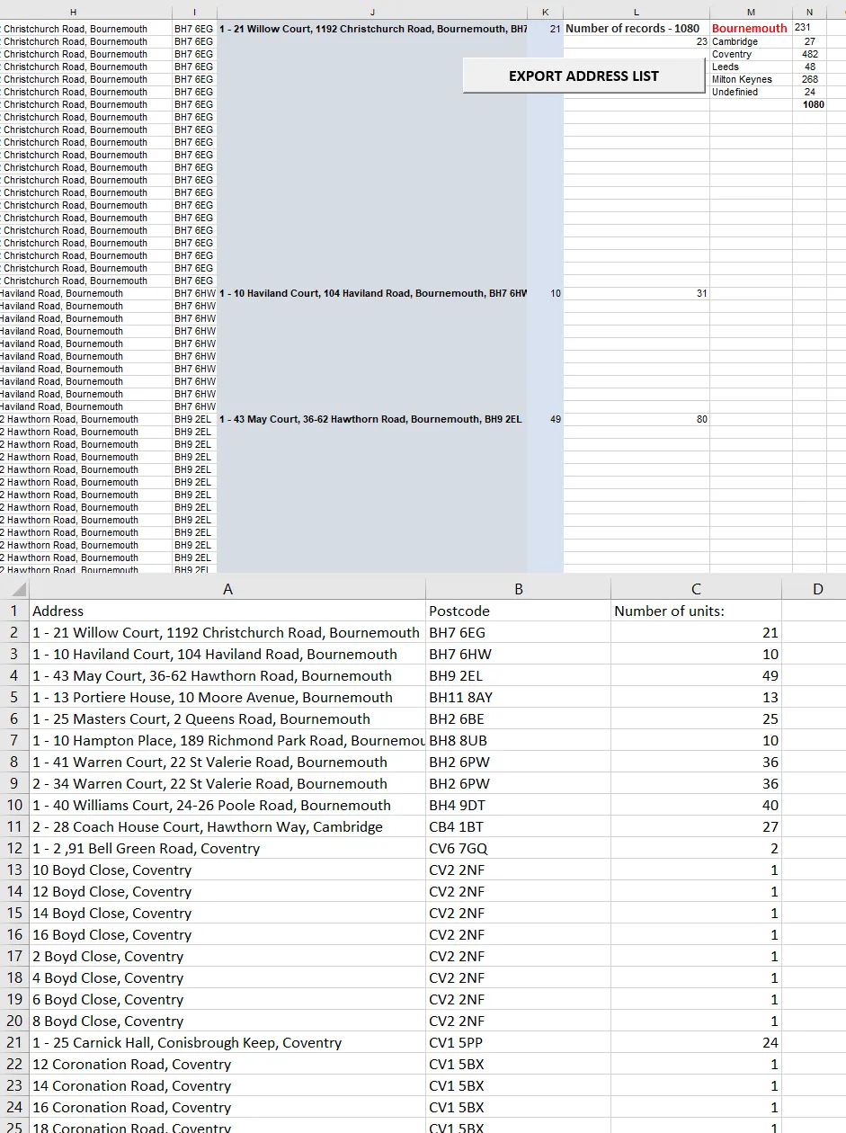
Pic. 14 Our final address list is in the main file and its new product is exported as the .csv file.
5. SUMMARY
I am attaching the file I was working on. I hope it will be helpful for you. These are my approaches, which are not the only ones existing. Both within the VBA code and Excel formulas we have a lot of ways to solve it. If you can do it quicker, I am open to discussing it in the comments or via contact. The major problem here is the SUBSTITUTE() function in column B, as we don’t know certainly what part of the string is going to be removed by us (we don’t know the city districts in advance) unless we deal with the same area, then it can be done quicker. Despite the tremendous work done, I could reduce the total address list from 1080 to around 460 records. It’s very helpful, especially for further geocoding purposes, where the total amount of inputs is usually limited. The file I was working on includes all the formulas used and discussed in this article. If you are lost, you have the stuff to refer to. The new .csv file being an output of my tremendous work here is finally the data, which can be next used for batch geocoding, plotting in the JavaScript API interactive maps, or other interactive map builders, where all these addresses can be easily populated.
The link to my Excel address list is here (file A and file B).
I hope the next part of this article, sacrificed on the PostgreSQL language will provide a quicker solution.
Mariusz Krukar
Links:
- https://www.ablebits.com/office-addins-blog/2016/11/16/excel-trim-function/
- exceljet.net/formula/remove-text-by-matching
- https://exceljet.net/formula/get-last-word
- https://www.extendoffice.com/excel/formulas/excel-get-last-word.html
- https://exceljet.net/excel-functions/excel-right-function
- 8 Ways To Split Text By Delimiter In Excel
- How To Extract First Or Last Two Or N Words From Text String?
- https://excelnotes.com/how-to-extract-the-first-two-words/
- http://howtouseexcel.net/how-to-extract-the-first-two-words-in-a-cell
- https://www.excelhow.net/how-to-extract-text-after-first-comma-or-space.html
- https://www.excel-easy.com/examples/substring.html
- https://howtouseexcel.net/how-to-extract-words-before-and-after-a-comma
- https://www.exceltip.com/excel-text-formulas/remove-unwanted-characters-in-excel.html
- https://www.extendoffice.com/documents/excel/3639-excel-extract-part-of-string.html
- https://www.ablebits.com/office-addins-blog/2016/06/01/split-text-string-excel/
- https://www.extendoffice.com/documents/excel/1783-excel-remove-text-before-character.html
- https://www.ablebits.com/office-addins-blog/2017/11/22/excel-extract-number-from-string/
- EXCEL ROW() function spec
- https://www.ablebits.com/office-addins-blog/2018/07/18/excel-convert-text-to-number/
- Calculate the smallest or largest number in a range#
- https://exceljet.net/formula/count-cells-that-contain-specific-text
- https://www.exceltip.com/other-qa-formulas/get-the-row-number-of-the-last-non-blank-cell-in-a-column-in-microsoft-excel.html
- https://exceljet.net/excel-functions/excel-iferror-function
- https://www.techrepublic.com/blog/microsoft-office/how-do-i-reference-cells-in-excel-with-a-countif-condition/
- https://docs.microsoft.com/en-us/office/troubleshoot/excel/formulas-to-count-occurrences-in-excel
- https://exceljet.net/excel-functions/excel-if-function
- https://exceljet.net/excel-functions/excel-indirect-function
- https://academy.datawrapper.de/article/89-prevent-excel-from-changing-numbers-into-dates
- https://www.automateexcel.com/vba/insert-row-column/
- https://support.microsoft.com/en-gb/office/stop-automatically-changing-numbers-to-dates-452bd2db-cc96-47d1-81e4-72cec11c4ed8
- https://exceljet.net/formula/cell-contains-specific-text
- https://www.ablebits.com/office-addins-blog/2020/10/22/excel-if-wildcard-statement/
Forums:
- https://stackoverflow.com/questions/43536646/delete-specific-words-from-a-string-of-texts-in-excel
- https://stackoverflow.com/questions/16490815/multiple-use-of-substitute-function-but-it-should-combine-the-results-in-one-col
- https://stackoverflow.com/questions/16104143/what-is-the-formula-to-keep-first-two-words-in-a-cell-over-excel
- https://www.mrexcel.com/board/threads/extract-first-two-words-of-a-cell.384215/
- https://stackoverflow.com/questions/43802036/remove-last-two-characters-in-cell
- https://stackoverflow.com/questions/61837696/excel-extract-substrings-from-string-using-filterxml
- https://stackoverflow.com/questions/47031077/how-to-delete-empty-cells-in-excel-using-vba
- https://stackoverflow.com/questions/14759174/split-address-field-in-excel
- https://stackoverflow.com/questions/10142448/excel-2007-vba-formula-with-quotes-in-it
- https://www.mrexcel.com/board/threads/trim-column-in-vba.1010210/
- https://stackoverflow.com/questions/2813925/how-to-get-the-path-of-current-worksheet-in-vba
My questions:
- https://stackoverflow.com/questions/61916476/excel-if-statement-for-trim-function
- https://stackoverflow.com/questions/65626333/excel-extract-one-word-from-the-any-part-of-the-string
- https://stackoverflow.com/questions/65899216/excel-extract-2-words-or-more-from-the-middle-of-the-string
- https://stackoverflow.com/questions/65955114/vba-excel-if-condition-for-splitting-address-columns
- https://stackoverflow.com/questions/65978311/vba-excel-export-the-file-as-csv-with-keeping-data-in-the-proper-columns
- https://stackoverflow.com/questions/65979769/excel-combination-of-isnumbersearch-with-concatenate-function?noredirect=1#comment116679263_65979769
Youtube:
https://www.youtube.com/watch?v=-f0kBpKKtSQ&ab_channel=MorryEghbal