Great American Eclipse visible from Europe

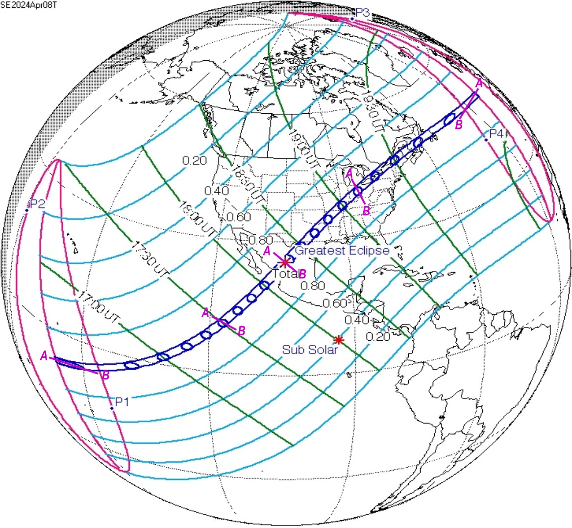
This is another lengthy text summarizing the solar eclipse from a scientific perspective. This time, it’s focused on the visibility of the Great American Eclipse in Europe. By understanding the Great American Eclipse, we mean the totality visible from North America on April 8, 2024. Notwithstanding the partial phase, which could be, at least theoretically, observed from many regions of Western Europe, we should indicate the areas lying within the rough extension of the totality. There are at least a couple of articles that discuss this particular matter, especially concerning the optimal observation window for the 12P Pons-Brooks comet, as well as a thorough analysis of all relevant circumstances, such as weather prospects and light pollution. They indicate plans and prospects of this celestial event. Now, as it has become history, it’s time to share what has undoubtedly been observed and how. Most importantly, the observation dispelled some doubts raised in previous articles. 

1. WEATHER CONDITIONS

The weather in Western Europe in early April is generally poor as the weather pattern transitions from winter to summer.  The absence of pressure area dominance characterizes this period, as the Icelandic Low weakens and the Azores High strengthens.  The significant influence of the Gulf Stream is spread evenly across all the areas considered for this observation. The proximity of all the lands to the Atlantic Ocean means that the rain takes hold, and the weather pattern can change rapidly. It doesn’t change the fact that some situations with clear skies and good visibility can occur, but they’re mostly unstable and don’t last long. Generally, the chance of good weather ranges between 40% in the north and approximately 50% in the south of the considered area. The weather prediction in detail was discussed before the eclipse expedition on this website, dedicated to all the eclipse events observable in Europe by 2030. Here, it’s time for the confrontation of the long-term weather prediction with the weather observed on the eclipse evening. There are a few disparities whose explanations can be valuable towards further planning of eclipse expeditions. At the outset, let’s examine the Ogimet and other weather data archives suitable for the eclipse evening in Western Europe (Fig. 1).

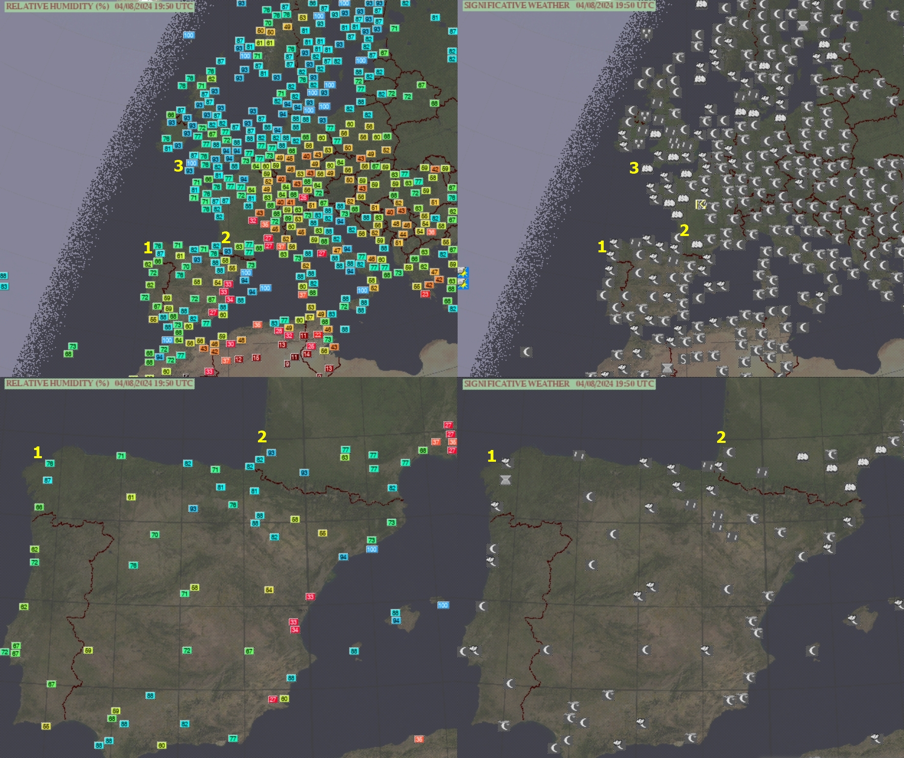
The evening of April 8, 2024, was predominantly rainy in western Europe. Even where the clear gaps in the sky were visible, the level of humidity was very high. For the 3 example locations considered in this long text, the best weather was in northwestern Spain. It was straight after the influence of humid maritime polar air mass, which featured a lot of advective clouds, bringing heavy rainfalls occasionally. The maps, surprisingly, show the clear skies above the western coast of France, which, at the time of the eclipse culmination, were located right at the back of the cold front. By examining other archived weather data from the evening of April 8, 2024, it appears to show a significant gap in clear skies above Nouvelle Aquitannie at late dusk (Pic. 2), although this discrepancy may not be accurate enough to account for potential eclipsed twilight observations.

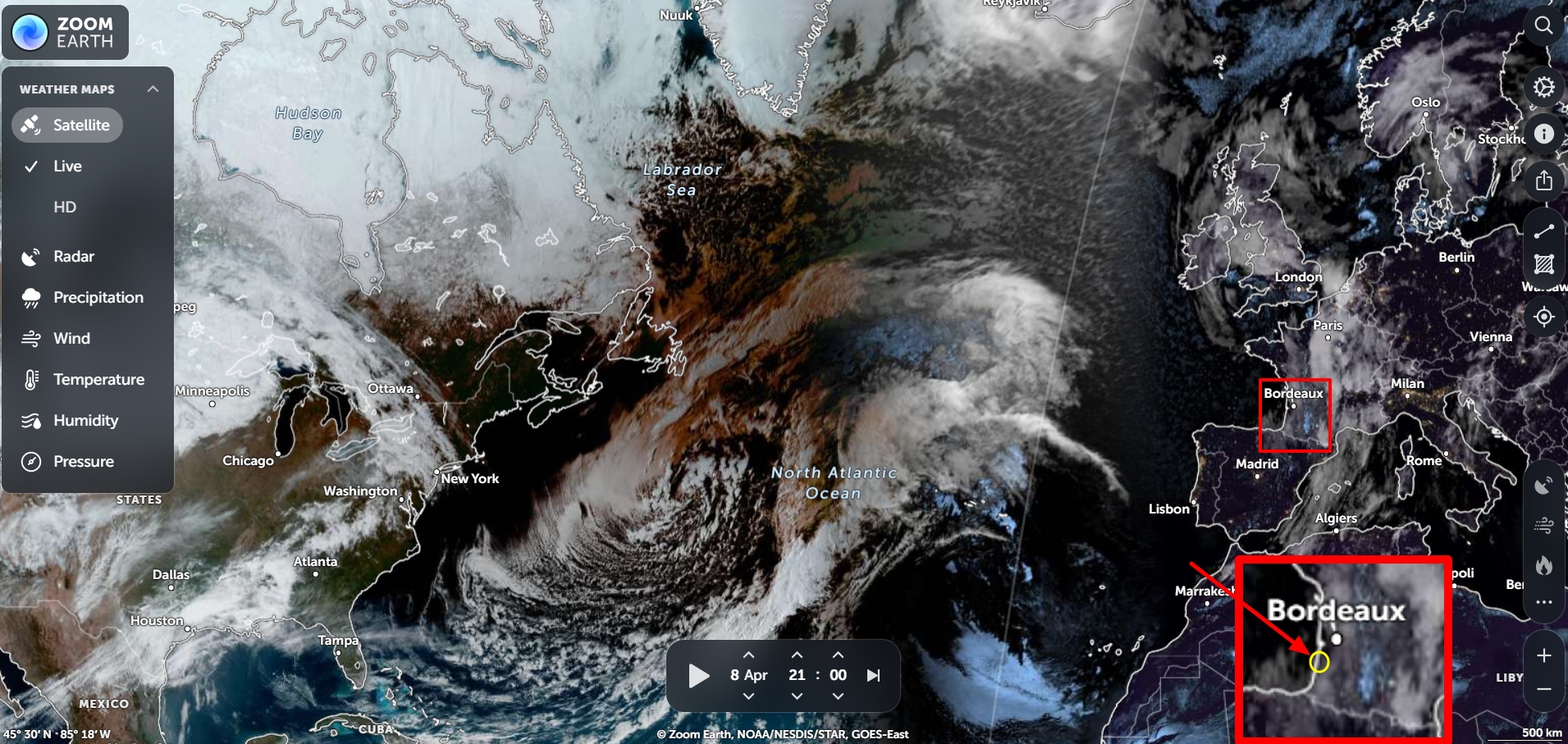
According to the zoom.earth satellite imagery, there was a serious clear section of the zenith sky entering western Nouvelle Aquitannie around 21:00 local time (Pic. 3), but because it was followed by the tail of high-level clouds backed by the advective thunderstorm cloud banks the western and northwestern horizon was presumably obstructed. The clouds were moving quite rapidly eastwards, leaving the same weather pattern behind as observed a bit earlier at Bretagne, Bay of Biscay, and north Galicia.

The worst weather, both predicted and observed, was in the southwestern part of the UK, considered the third venue, with the best visibility of the 2024 total solar eclipse below the horizon. The satellite image above shows, in fact, quite similar weather conditions to Nouvelle Aquitaine, where potentially, some clear sections of the sky could appear, but the crescent sunset, as well as further eclipse-induced twilight, wasn’t visible for sure. The core of the low-pressure area with high-level clouds was located at the Welsh coast, which was next moving southwards and southeastwards, covering the entire horizon from the western side. The best weather prospects, but beyond the range of eclipse visibility, occurred at Bretagne, which was relieved from the cold front much earlier. The twilight disturbance could be observed between the bands of heavy rainy clouds, whose presence and perspective against the local horizon excluded umbra visibility. In the worst position were people who embarked on the solar eclipse cruises running from the UK or Ireland.  They initially went to observe the totality at sunset in the mid-Atlantic, where another low-pressure area was passing by, bringing fully overcast skies and rain.
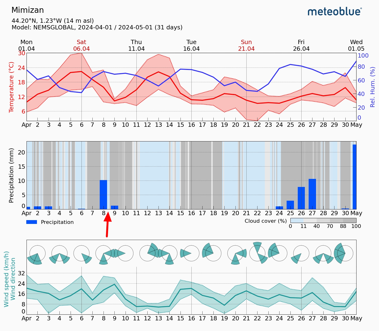
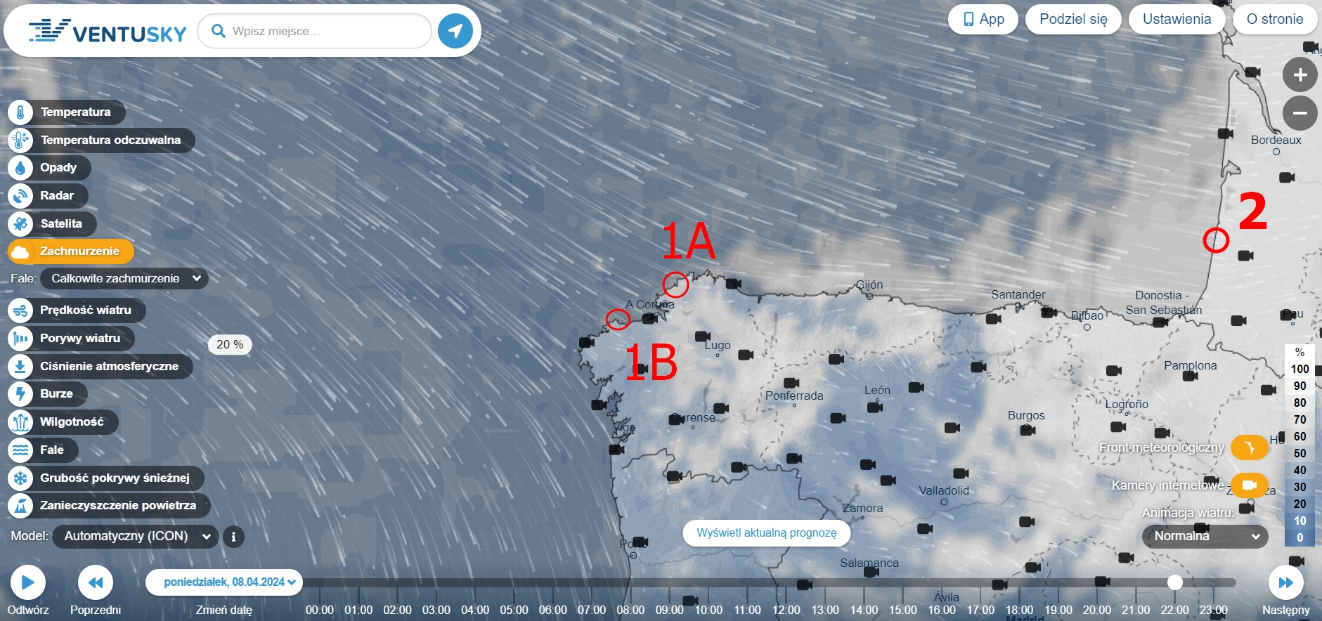
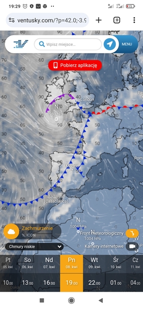
By returning to the location of Mimizan, which I had cordially considered as an alternative to Spain, I had a rare chance to observe the eclipse’s impact on astronomical twilight. However, the Ventusky.com service showed a fully overcast sky (Pic. 4).

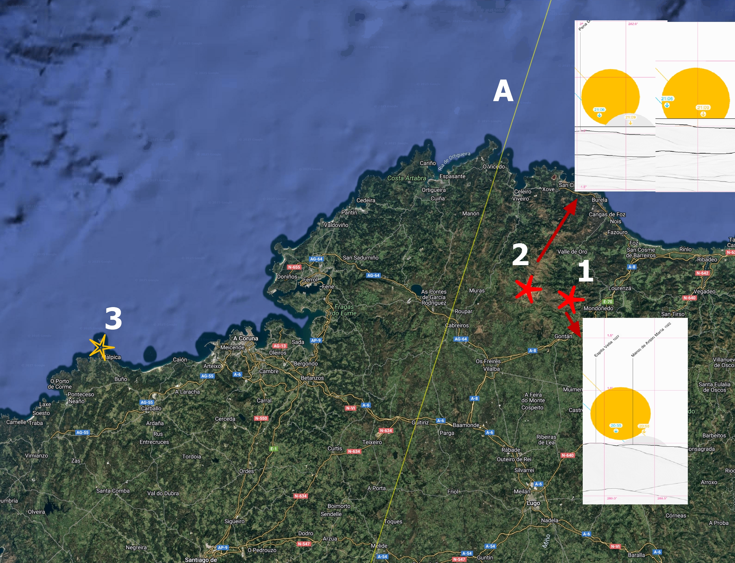
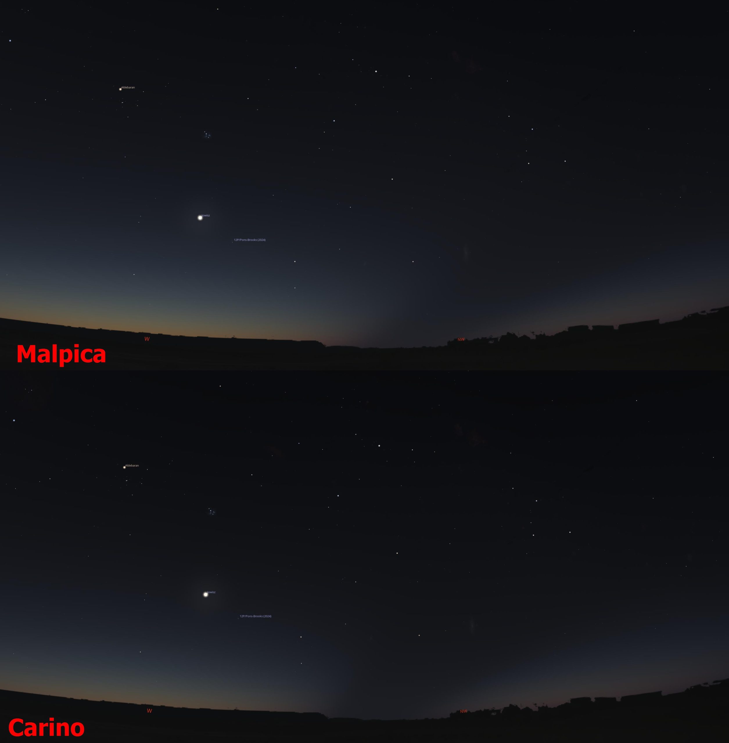
The weather in northwestern Spain was admittedly the best among several other locations in western Europe. However, this is a far-reaching general assumption based on the synoptic situation on April 8 late afternoon. The cold front swept rapidly across Galicia in the morning and midday hours, leaving clear but humid air in its back. Right after the high cloud deck, when the Sun starts shining, the wet ground starts to heat up and create the air updrafts. Just a short while after the Sun and cumulus clouds appeared, we could see larger clouds on the horizon, which began to bring heavy rainfall and occasional thunderstorms. They were mostly in banks, separated by large portions of clear skies. The situation persisted beyond the evening of the eclipse. According to the Weather & Radar application, Carino and Malpica towns were expected to have partially overcast skies around the moment of eclipse culmination (Pic. 5).

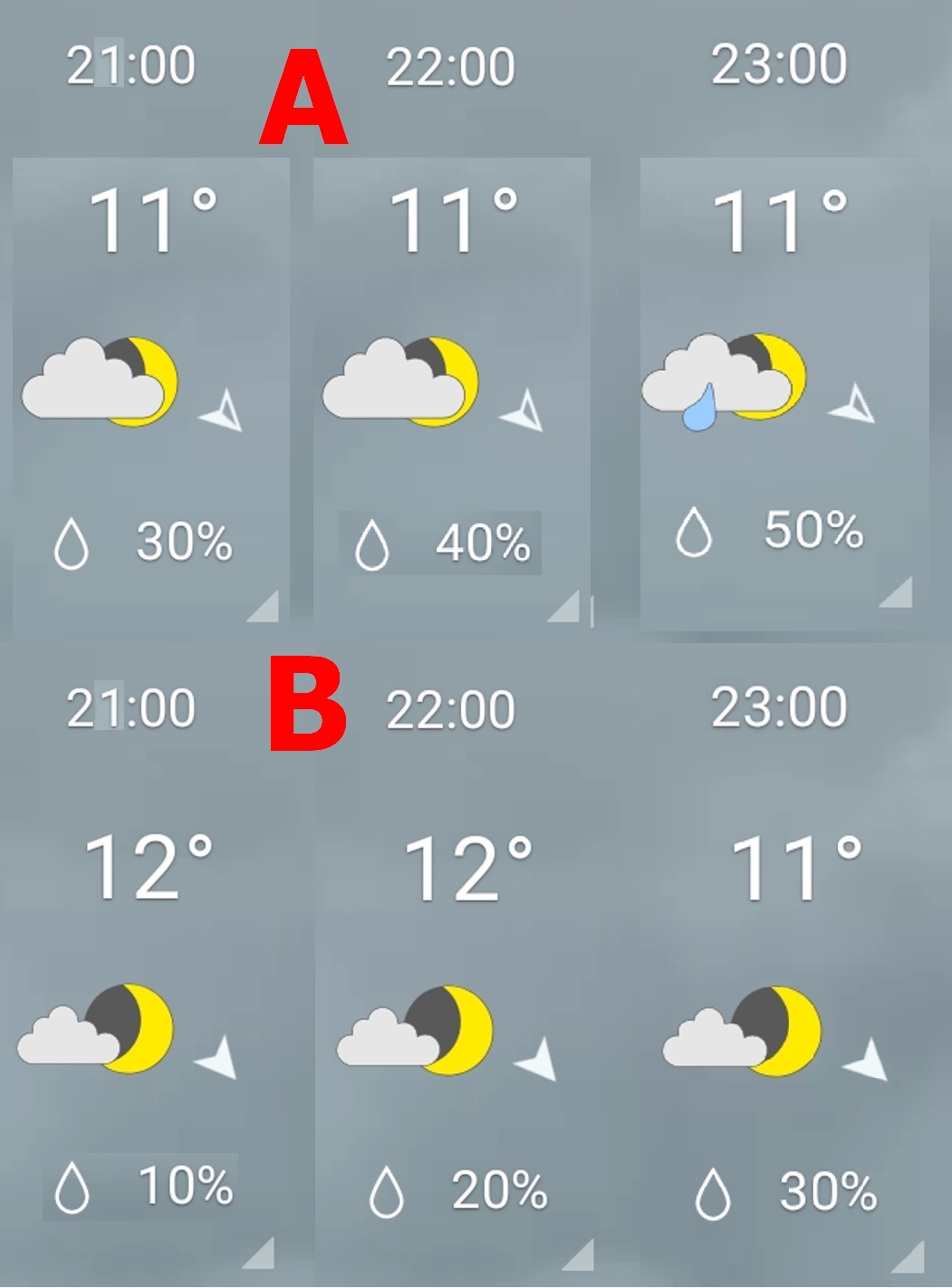
In both cases, the best weather was predicted between 20:00 and 21:00 local time, with slight deterioration in later hours. The town of Malpica had the best weather prediction among other locations considered in Galicia. Following the

The Weather & Radar application, which appears to work well in situations such as this, suggests that the scene could experience relatively clear skies with only light cloudiness, although any probability of precipitation would indicate more significant cloudiness in some areas. Conversely, the Carino region, especially its western part with the Garita de Herbeira cliffs, had the worst predictions, which stated rather cloudy weather with occasional clear gaps in the sky and a higher probability of precipitation. These two weather predictions (Pic. 5), combined with the archive data presented for Mimizan (Pic. 2), tie up one core thing! This is a proper understanding of weather prediction. Even if it’s correct for a specific location, it never covers the entire sky! Having the clear skies (or full “Sun”) predicted means that the near-zenith sky is clear, but the horizon skies are not necessarily clear. Since the near-zenith sky can be considered down to an altitude of around 20-30º above the horizon, the sky at the distant horizon will represent a different location with separate weather predictions. Considering Maplica, where many images below in this article show the weather on the evening of the eclipse, the horizon sky was almost fully overcast regardless of the weather prediction. The same would happen for Mimizan, and surely did, what can be concluded from the zoom.earth satellite imagery presented above (Pic. 3). Anyhow, this understanding of weather prediction is crucial not only for solar eclipses occurring very low above the horizon or their impact on twilight but also for long-distance observations. Therefore, when planning an observation such as this, it’s worth analyzing weather prediction not only in the place from which you are going to watch it but also in adjacent places towards the direction from which the event is going to be observed.

The next step is to analyze long-term weather satellite data for the observation location, specifically for a day on which the astronomical event is observed. Before April 8, 2024, observation in Europe, I compiled a detailed weather pattern based on the worldview.earthdata.nasa.gov service, as described here. The dark side of this analysis is the fixed time at which the imagery is taken. MODIS satellite imagery is produced daily, typically at midday or early afternoon. From the perspective of a morning or evening solar eclipse, this imagery isn’t reliable enough. The best example is shown below, where a comparison of cloud coverage against the April 8, 2024, MODIS satellite imagery is presented (Pic. 6).

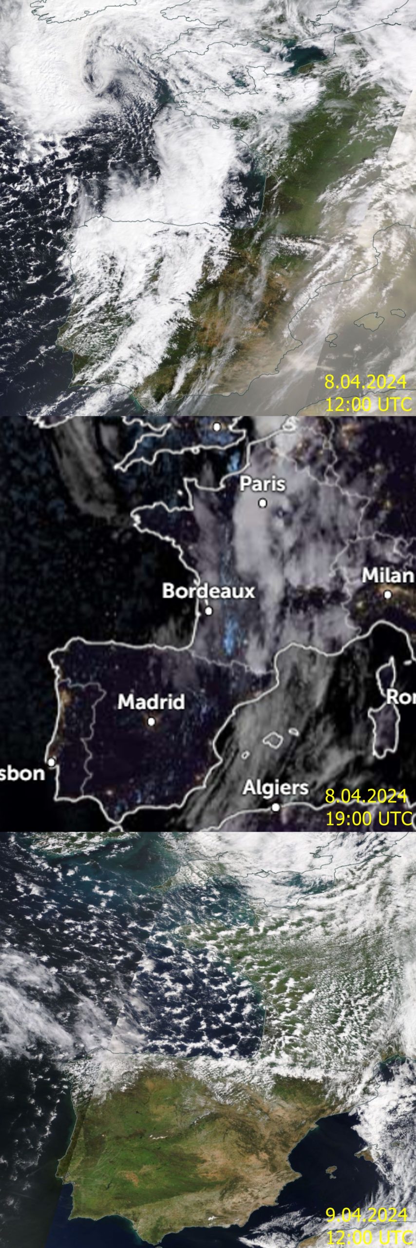
The cold front visible in the topmost image (Pic. 7) moved a few hundred kilometers eastward within just 8-9 hours. I hope to explain it in the future, but just for now, it’s essential to mention the various speeds of clouds, which are shaped by the type of surface. In this specific case, the frontal clouds were moving above the water surface, which typically moves at around 60 km/h. This is precisely where the difference between just several hours comes from. For further reference, situations like these should be carefully considered when planning your observation away from midday.

Lastly, let’s discuss the weather report at my observation site in northwestern Spain. By examining the image above, the cold front brought clear but humid air with numerous thundery cloud bands separated by vast, clear sections of sky (Fig. 7, 8). This type of weather means one thing: the horizon is fully obstructed by clouds, so observations of eclipses near sunset or sunrise are never possible.

The period of relatively good sunny weather lasts for about 30-45 minutes, then it turns around, bringing heavy rainfall and thunderstorms for the next half hour or so, as shown in the video below.

Thunderstorm in A Coruna, 7 hours before the eclipse culmination

The weather prediction for observing celestial events is like a rollercoaster. The specificity of this low-pressure area was an increase in humidity level near its center (Pic. 6), thereby reducing the chances of good weather around Carino. The screenshot below shows the situation around 2 hours before the eclipse culmination (Pic. 9).

The cloud banks are heading directly from the northwest to the Spanish shores. The video on the right displays a set of weather and radar screenshots collected over the last 6 hours of April 8th, when the eclipse occurred. There was quite a big difference in their intensity. Northern areas used to catch more developed thunderstorm systems, whereas in the south, they were a bit more dispersed. The most important factor in weather circumstances such as these is the surface. Since the humid air passes smoothly over the large water body, the situation dramatically changes as this air encounters the topographic obstruction. As a result, the air rises and condenses into the clouds. An observer watching the clear sky in front of his eyes might suddenly face freshly developed clouds right above his head, or earlier. The more intensive cloud development is characteristic of areas at higher elevations, directly facing the sea. The Garita de Herbeira cliffs were particularly prone to such results, so the topography factor was an additional reason for the significant increase in cloudiness. Conversely, the surroundings of Malpica, located at around 150 m above sea level, were much less affected by this weather phenomenon. It doesn’t change the fact that adjacent areas with massive highlands were catching much more clouds, which will be indicated in the following chapters.
The video below shows what the weather might look like in Carino (or Garita de Herbeira) compared to Maplica. The zenith sky was presumed to be clear at eclipse culmination, although the northwestern horizon could be purportedly obstructed by a large thundery cloud bank approaching the landfall. Moreover, the increase in clouds and precipitation can be noticed around the shoreline.

The animation of cloud banks moving over northwestern corner of Spain around the solar eclipse event on April 8, 2024. Various blue spots indicates the level of precipitation (Weather & Radar app).

2. OBSERVATION VENUE & EQUIPMENT

The first discussion about the solar eclipse was in the car rental office. They informed me that they are aware of the celestial event scheduled for Monday. At first, I thought that my web-based endeavors regarding encouraging people to watch the event below the horizon were successful. I was pretty much convinced to the eclipse event, when arrived on site north west of Malpica (Pic. 9) I was unable to set up at the very top of the hill. I was surprised to see several cars driving in the same direction to the top of the hill.

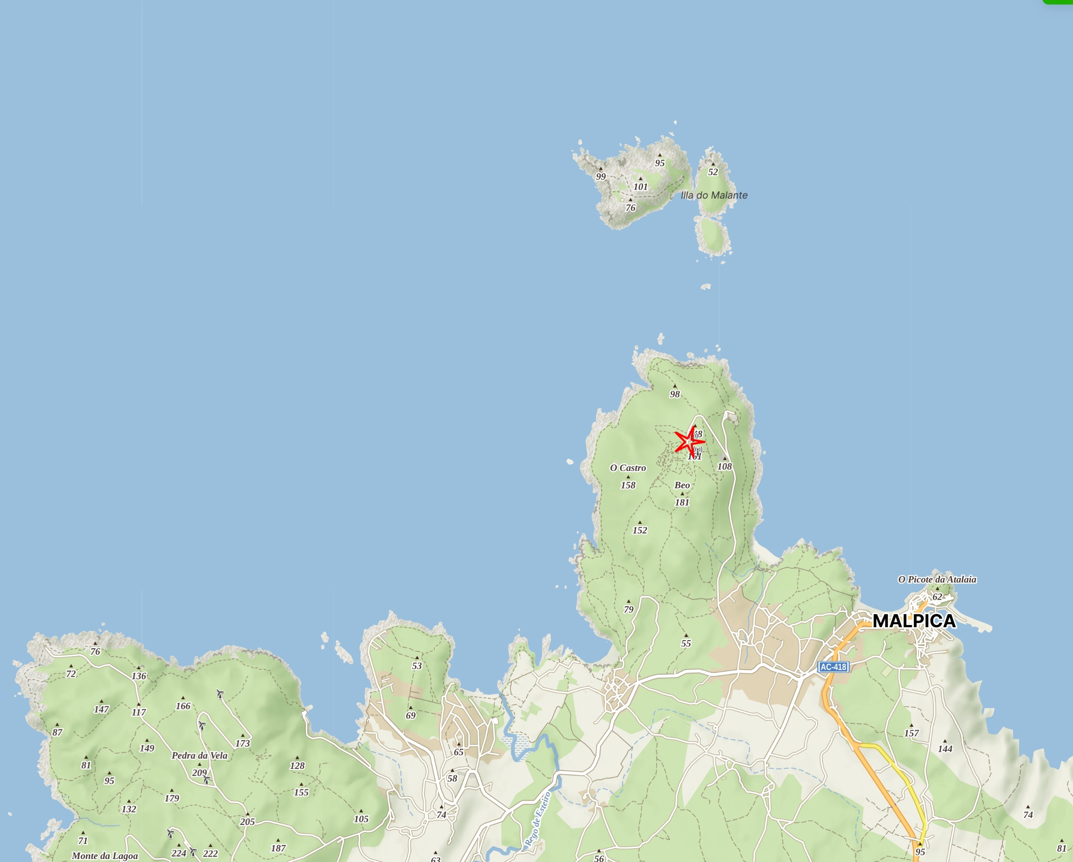
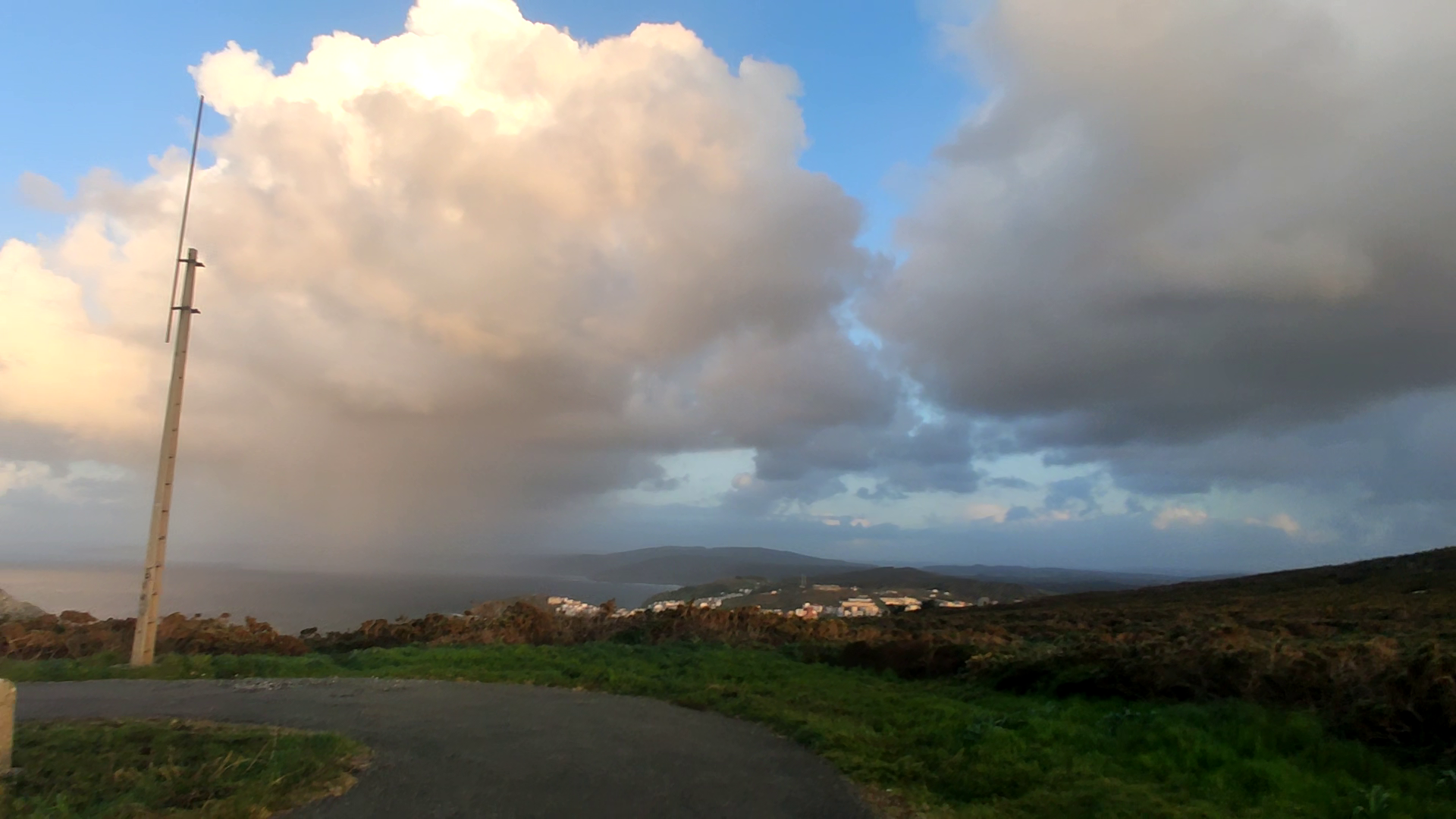
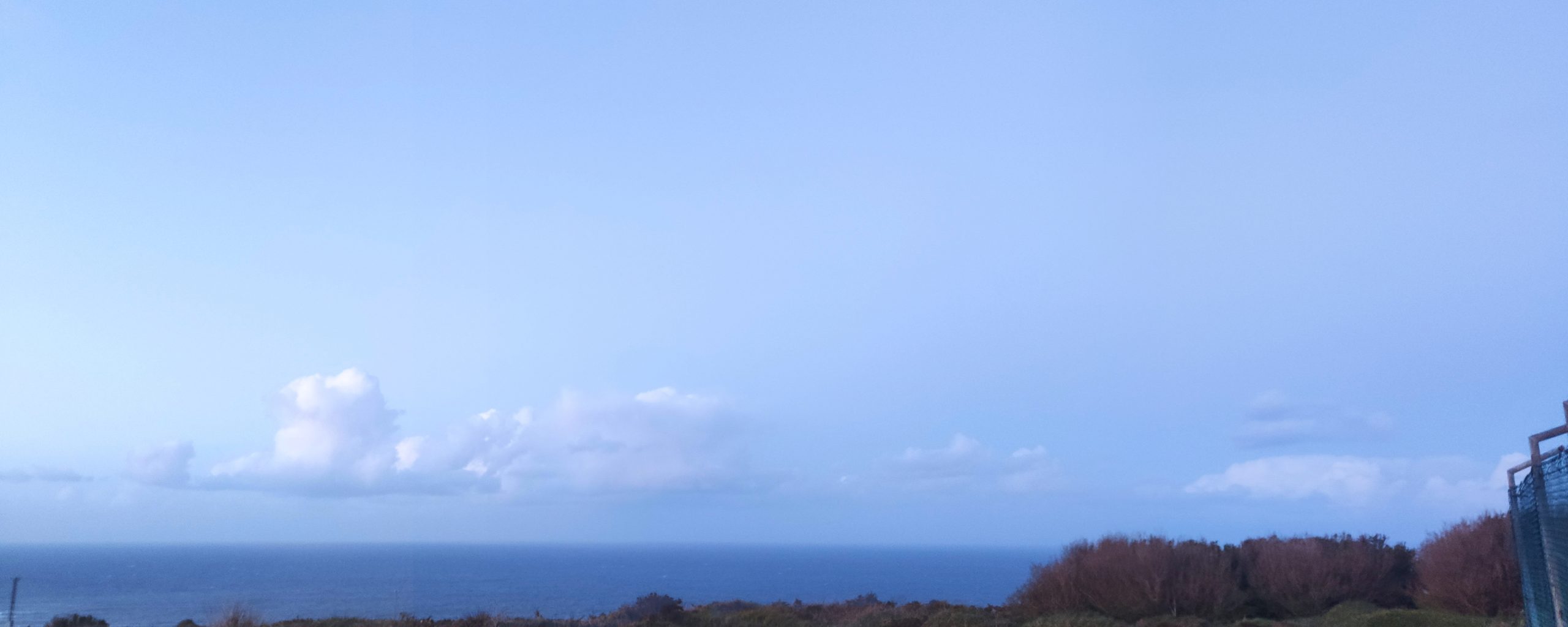
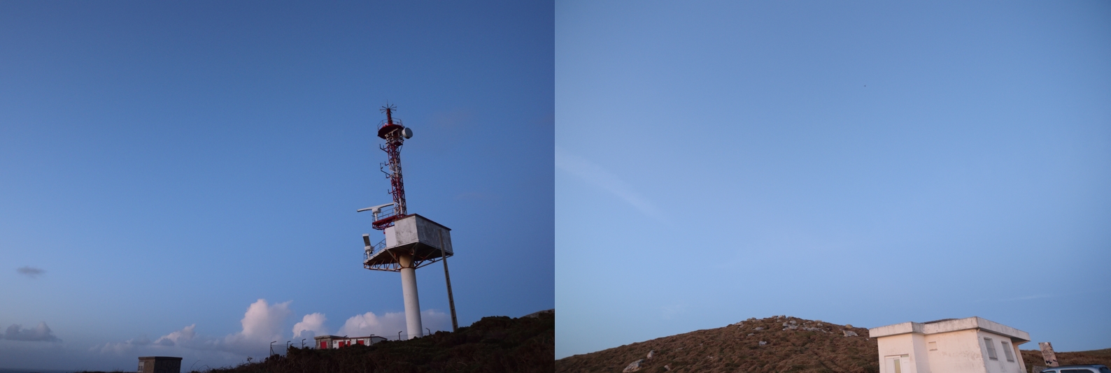
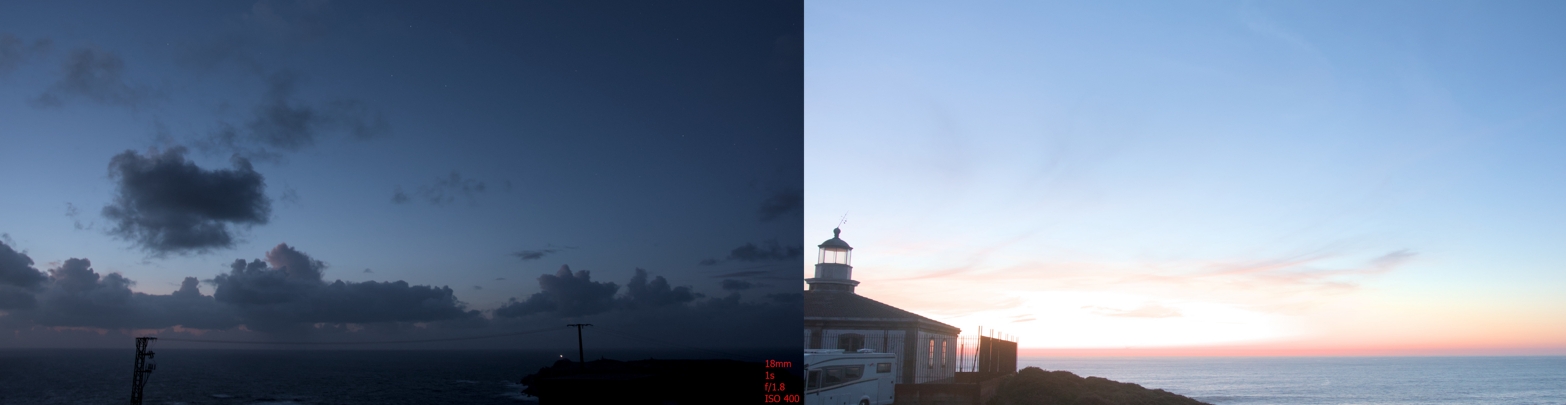
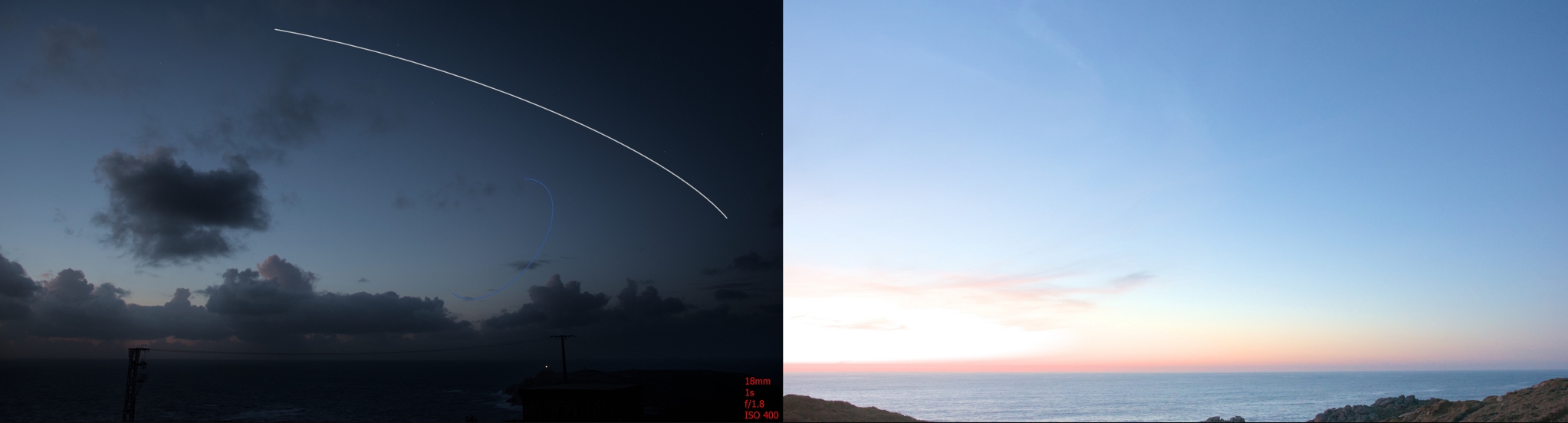
The hilltop was crowded with several people preparing for pictures, walking with their dogs, and strolling through the wet grasslands. The narrow road was busy with cars coming to the top. When I arrived, the weather started to improve as the most extensive clear section of sky approached the area (Pic. 10-13).

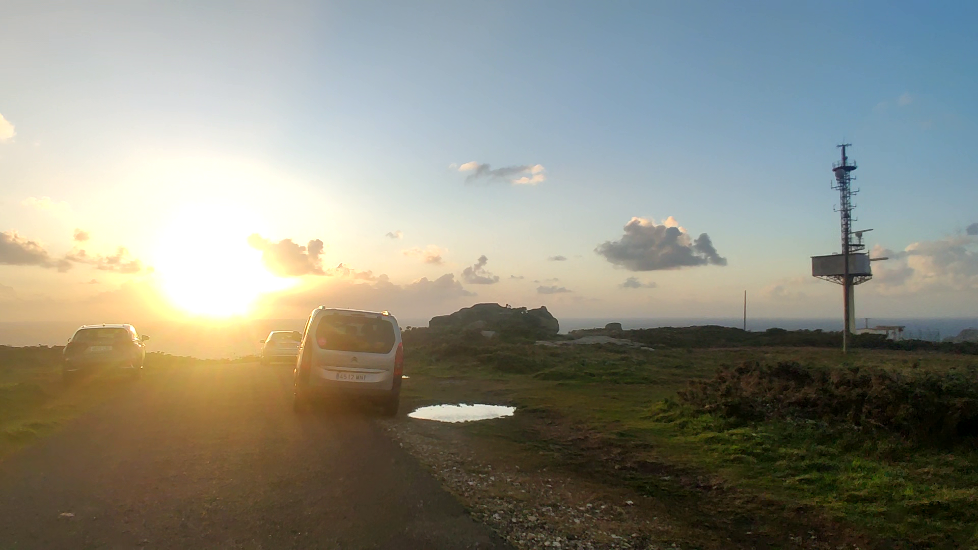
Unfortunately, shortly after the Sun went behind the clouds, people got into their cars and drove back. After a short while in the crowd, I was alone. In light of this situation, it wasn’t necessary to change my observation position as I located myself about 20m lower, just underneath the mobile transmitter.

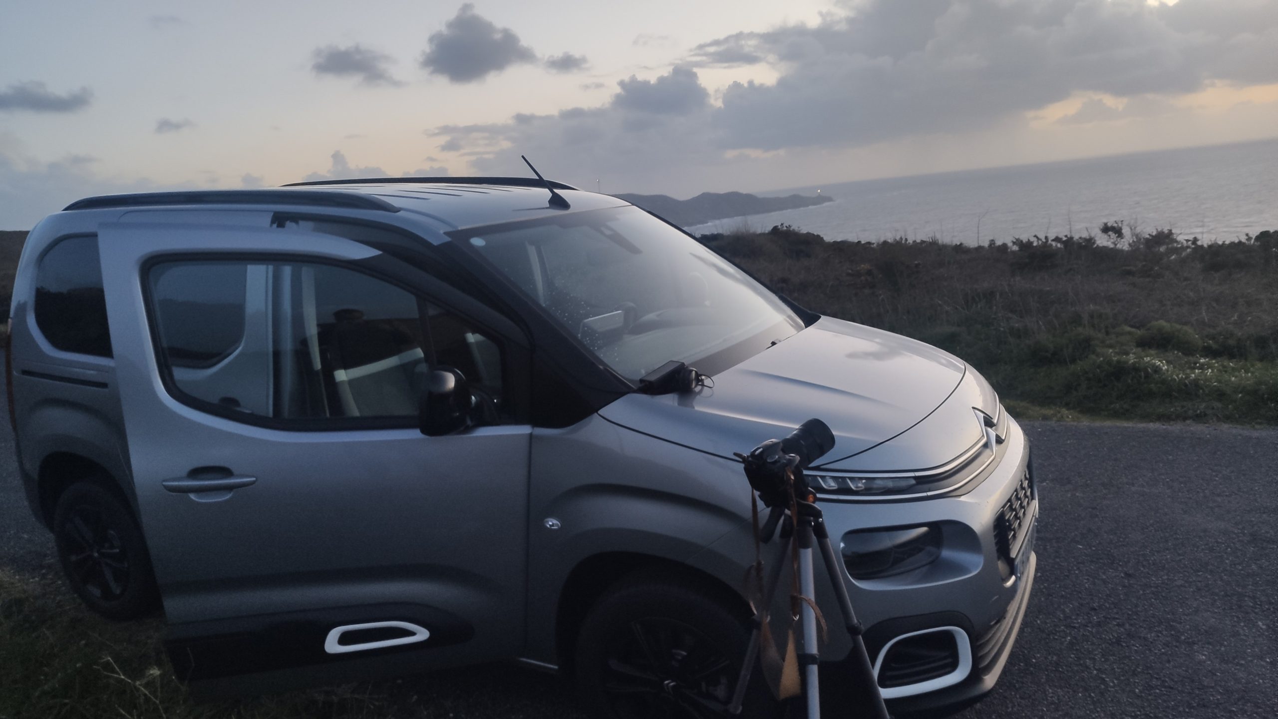
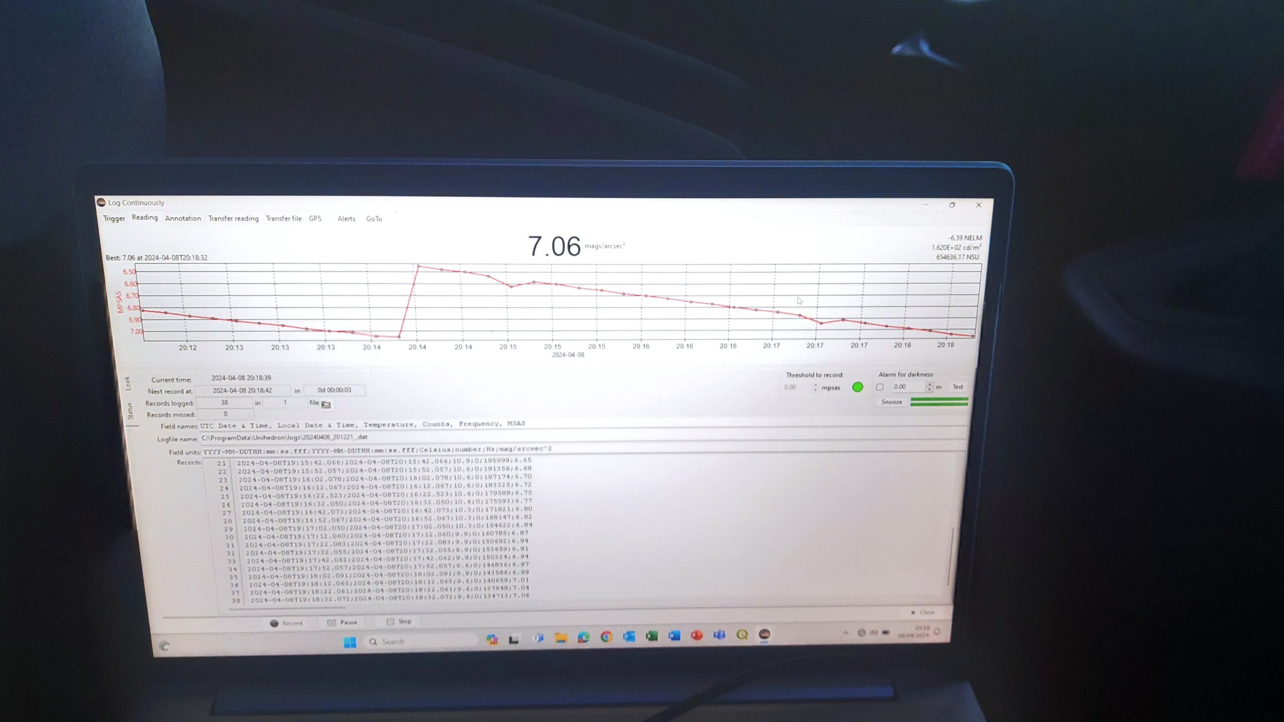
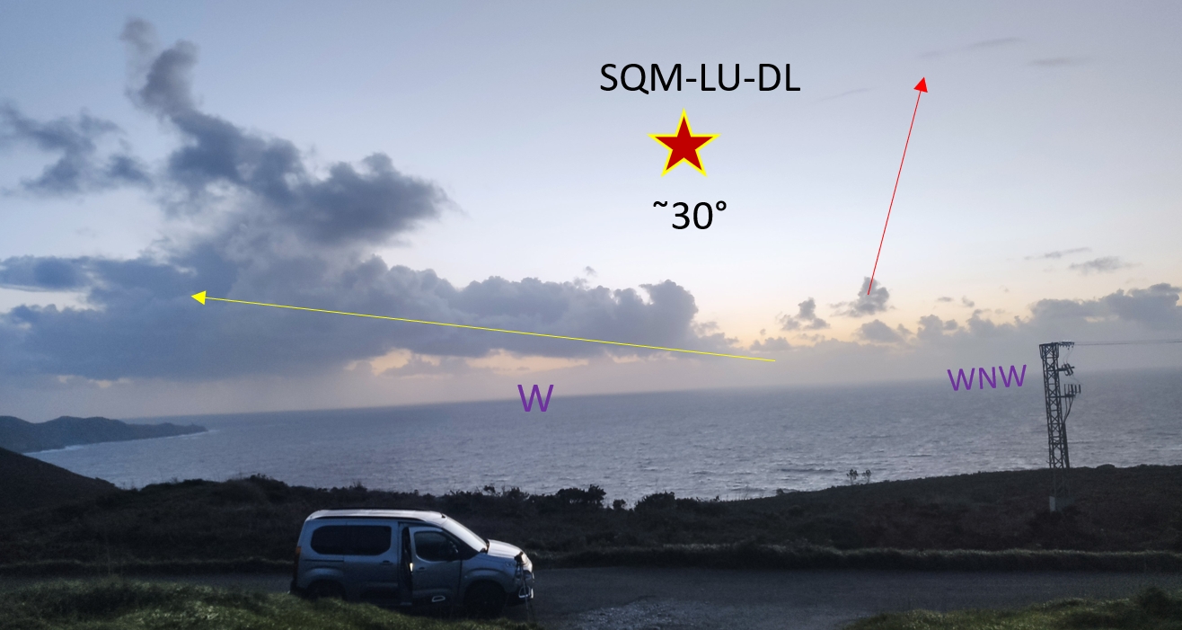
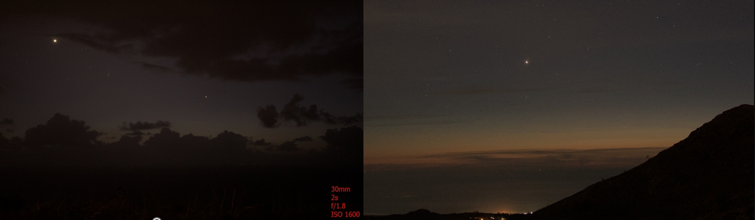
After the setup, I was ready for the observation around 10 minutes after catching a rather unsuccessful geometrical sunset. I used three devices. The first one was my phone, the Xiaomi Mi 9, which was able to capture simple images with random parameters, as shown above (Pics. 10-12). The second one was my DSLR camera – Nikon D5300 with the Sigma 18-35mm f/1.8 Art attached and the Tokina AT-X Pro 11-16mm f/2.8 DX II, optionally for wide-angle photography. My third device was Unihedron-LU-DL for sky surface brightness measurement set for 15s intervals and oriented at an altitude of approximately 30 degrees in the WNW direction (Pic. 13).

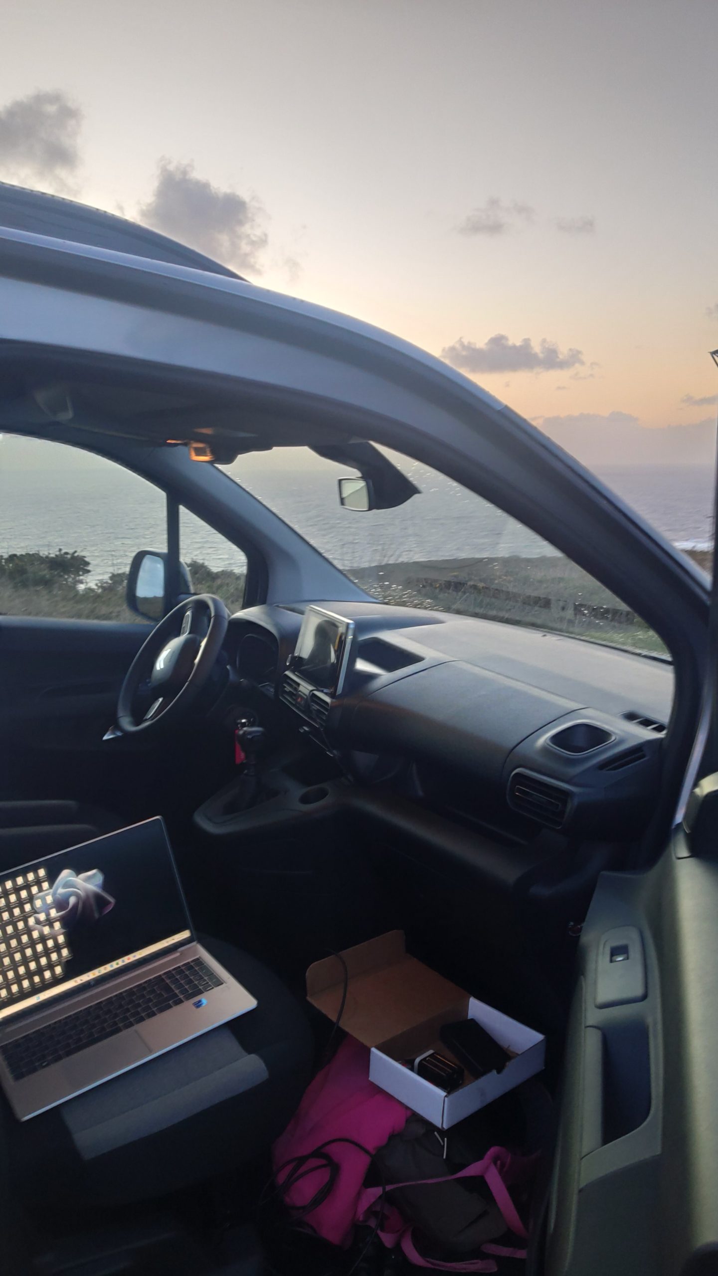
The Unihedron LU-DL device was directly connected (by the USB cable) to the HP laptop with the operating Unihedron application logger (Pic. 14-15).

 

 3. THE FIRST CONTACT AGAINST THE GEOMETRICAL SUNSET

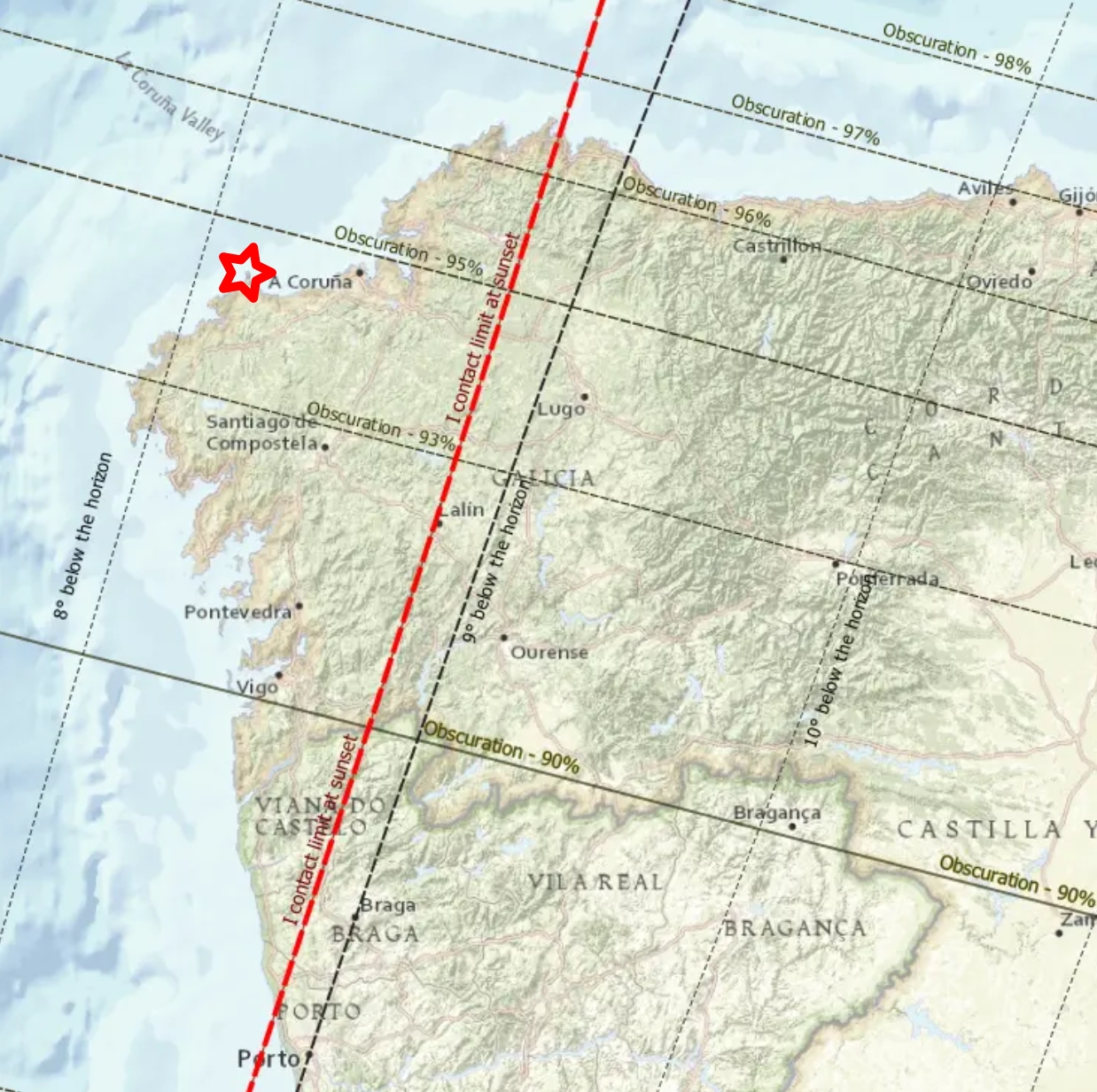
The very first aim of my observation was the sunset itself. My location was in the vicinity of the first contact limit at sunset, as the greatest obscuration physically possible to observe was about 4,5% from my area (Pic. 16).

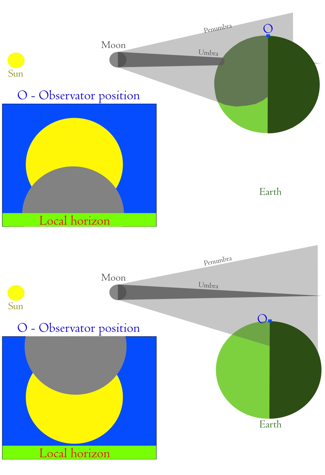
The geometrical limit of the first contact isn’t a trivial thing to understand. It’s because the line presented on the map marks the beginning of the eclipse when the center of the Sun is on the horizon, additionally, without the refraction. Even so, we need to understand the sun as a disk. Since the apparent diameter of the Sun is not zero (Meeus, 1997), there is a complication in understanding this limit. This is explained well in the figure below (Fig. 17).

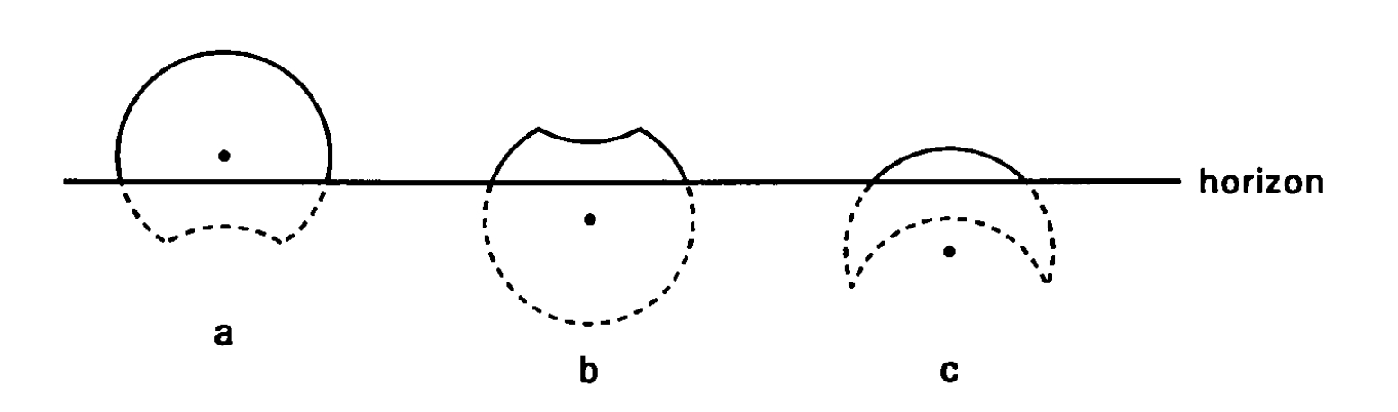
The situation in which the eclipse is to be observed at 1st or 4th contact (consequently at sunset or sunrise), the most appropriate will be the first situation (Pic 17a) at which an observer standing roughly on the line marking the limit of 1st contact won’t see the eclipse at all. Since the center of the solar disk is considered the limit, the eclipse from that position will last only half of sunrise or sunset, which begins or ends, is defined by the upper solar limb’s appearance on the horizon. During this relatively short time, the eclipse progresses, but at the bottom side of the limb, it is invisible to the observer. Considering my situation, when the Sun was eclipsed by 4.5%, “a” is an adequate situation. If I were placed several hundred kilometers west, then “c” could be applicable. These two situations have the exact position of the Moon’s disk, which moves more slowly than the Sun in the sky. From the perspective of someone who watches the event before sunset, the Moon appears to come from the “bottom” as it sets, more slowly than the Sun. Turning this situation upside down by placing an observer near the sunrise, the lunar disk will also be observed from the “bottom”, but because it rises more slowly, the eclipse progress is monitored in reverse sequence. Another consequence of this geometry is the visual position of the solar crescent. Under specific circumstances, when the Sun is low above the horizon, the lunar disk can be placed inside, creating a solar crescent with both horns down. It means that the central eclipse occurs somewhere on Earth, determined by the path. The situation b is opposite and represents the moment at which the eclipse finishes at sunset or begins at sunrise. Because the position of the lunar disk is external here, making the Sun’s crescent with both horns up, an observer sees the greatest eclipse on the Earth’s surface. No central eclipse takes place on Earth. The explanation of the sketch above (Fig. 17) is illustrated in another sketch below (Fig. 18) for better understanding.

In my situation in Spain, I could consider the example of venues located close to the eclipse limit, which passed across the Xistral mountain group—the westernmost part of the Cordillera Cantábrica range. The altitude of over 1100m.a.s.l. additionally contributed to the eclipse’s limited visibility because of the horizon dip of approximately 1°, not to mention the astronomical refraction, which also committed to the 1^st contact limit of visibility. The image below illustrates the best relationship between the limit of eclipse visibility, as determined by Xavier Jubier, and the topographical circumstances (Pic. 19).

The differences in visual obscuration at the beginning of sunset can be significant in relation to local topography. What is most curious is that by the hypothetical moving of the observer to the adjacent mountain ridge located just a few kilometers eastwards (1), we are “losing” the eclipse completely.
There is another aspect worth attention to when looking at the sketch above (Pic. 17). The crescent is oriented parallel to the horizontal line with both horns at the same angular distance to the horizon. It’s an ideal representation of the circumstances, which happen very rarely. Namely, we could see them when an observer is standing roughly at the centerline, and the ecliptic line is perpendicular to the horizon. It’s typical for the lowest latitudes. Analyzing the situation in northwestern Spain, we had at least two additional elements that made the position of the solar crescent slightly different. The first one is the latitude, at which the ecliptic line is never perpendicular to the horizon. The second one was the placement off the centerline, which resulted in no central movement of the umbra on the solar disk. The way the Moon’s disk moves across the Sun during the entire eclipse isn’t straightforward and requires additional explanation, which I will provide in the future.

Observation from my location was unsuccessful due to cloud obstruction on the horizon. As explained above, it’s typical for the weather pattern to occur on the evening of the eclipse. The Sun was visible well shortly before the 1^st contact (Pic. 20)

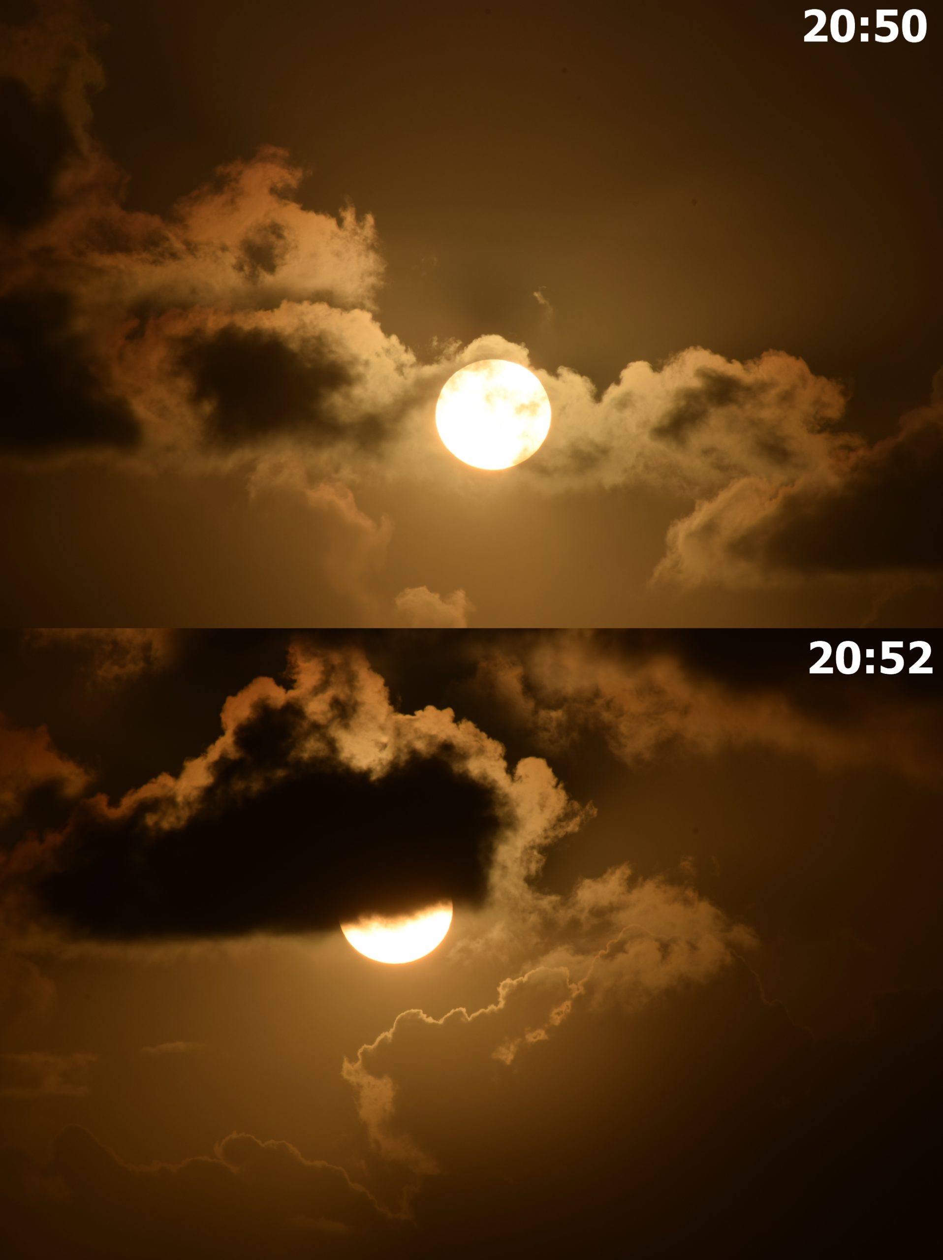
Unfortunately, later, the bank of clouds was too large, and the 1^st contact was missed by everyone located in that place. I am convinced that nobody took an image of the eclipsed Sun from there because I saw nobody with a DSLR camera. I was only a little fortunate to see a small part of the eclipsed Sun in the thin hole between the clouds (Pic. 21). I am sure it was a pretty large section of clear sky, which was flattened entirely due to the viewing perspective. This is why the observations of celestial events near the horizon are neuralgic. Even if cloudiness doesn’t prevail, the horizon might be obstructed. It explains why the conditions of watching the total solar eclipse of August 12, 2026, from the Balearic Islands will be tricky.

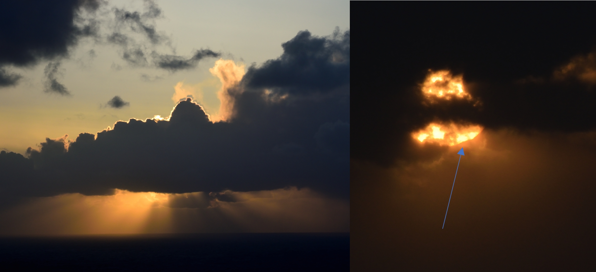
The eclipsed Sun was visible shortly after the 1st contact for literally tens of seconds between two cloud banks. If the horizon sky was clear, I could see a marvellous eclipsed sunset accompanied by some remarkable optical phenomena. Fortunately, it was just one unsuccessful bit of the whole observation that evening.

4. LIMB DARKENING EFFECT

Because the eclipse started shortly before sunset, the twilight was affected by this celestial event from the very beginning, even if it wasn’t noticeable by the observer at all. Except for the Moon’s presence on the solar disk, a small partial solar eclipse is believed to be unnoticeable to observers in terms of various optical phenomena. It may be especially applicable in situations where the eclipsed Sun goes beneath the horizon, leaving “normal” twilight behind. The optical contribution of the eclipse event isn’t detectable by the observer or its instrument unless the observation is repeated in the same manner for non-eclipse conditions. That’s why the way of watching the solar eclipse below the horizon was proposed in this article. However, it could also be applied within the geometrical limit of the eclipse for monitoring the changes that contribute to the sky and scene. Of course, as mentioned multiple times in various texts, the drop in light level will be the easiest thing to notice; however, much more interesting is the spectral disturbance caused by the eclipse event. This is the limb darkening effect, which comes from non-uniform sunlight. In a recent article, the phenomenon was explained in detail concerning the eclipsed Sun visible to the observer. Depending on the Sun’s altitude above the horizon, the circumstances of Rayleigh scattering modified by the limb darkening effect will have an individual character. However, the limb darkening effect itself can be treated in a standard way, especially when the solar activity and other factors are neglected. The general influence of limb darkening on the sky is illustrated concisely in the graph below (Fig. 22).

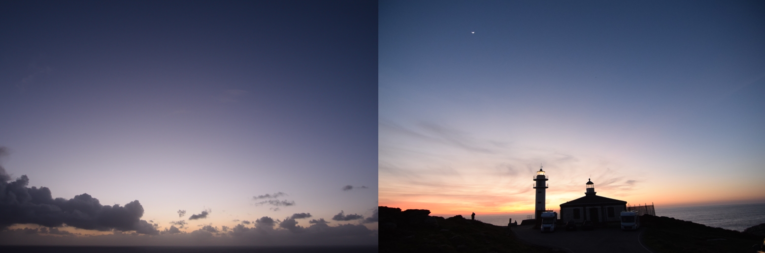
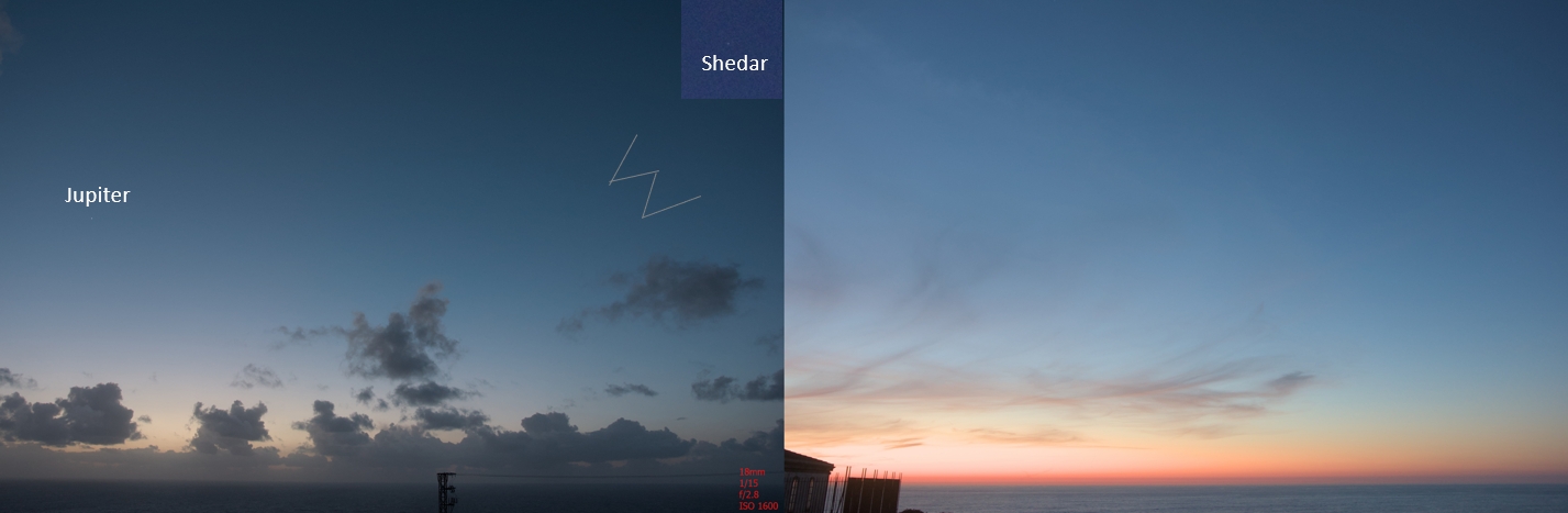
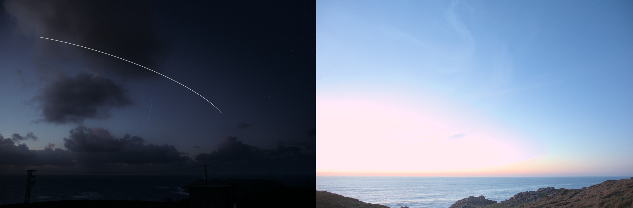
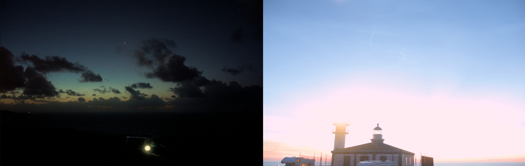
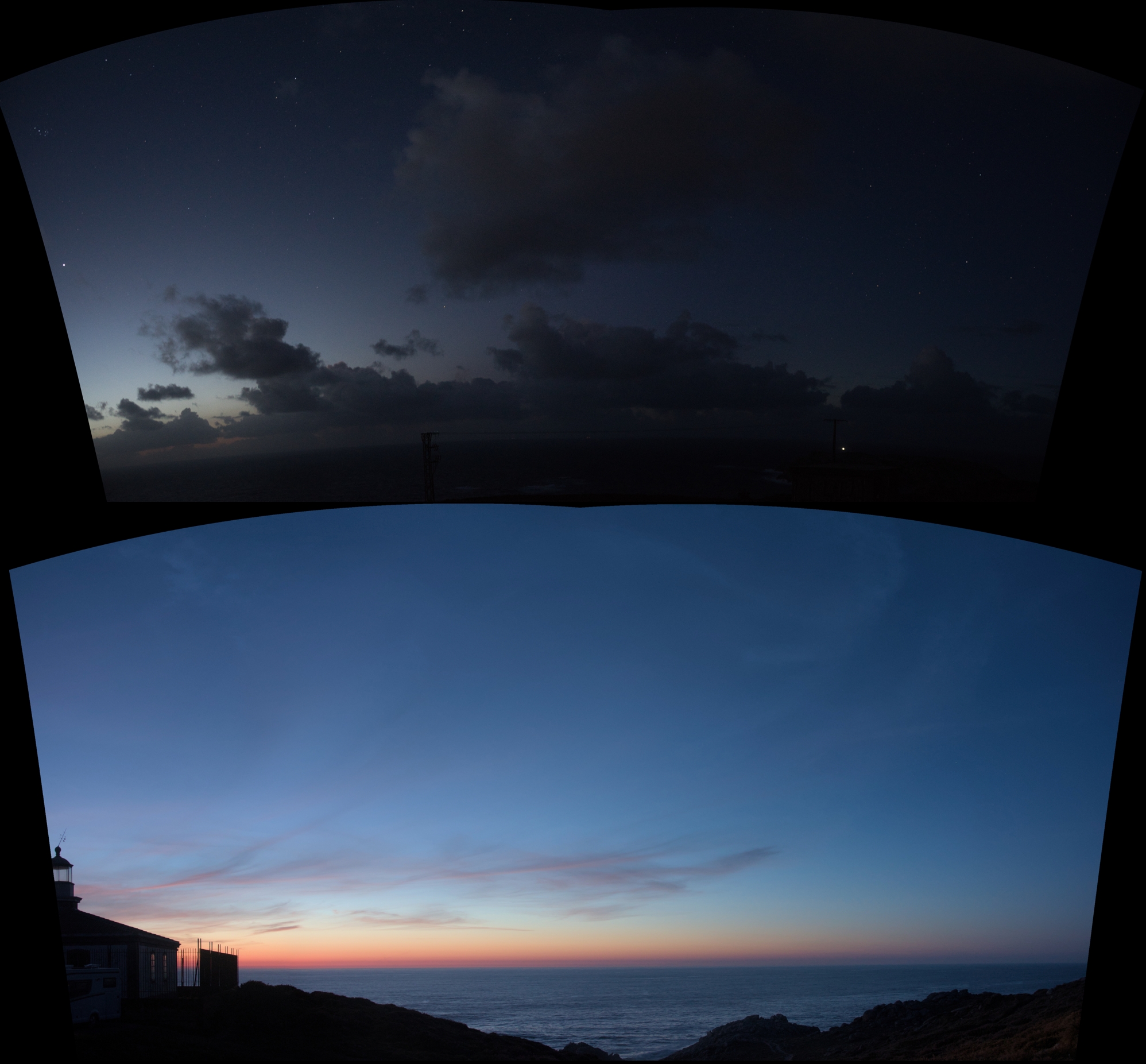
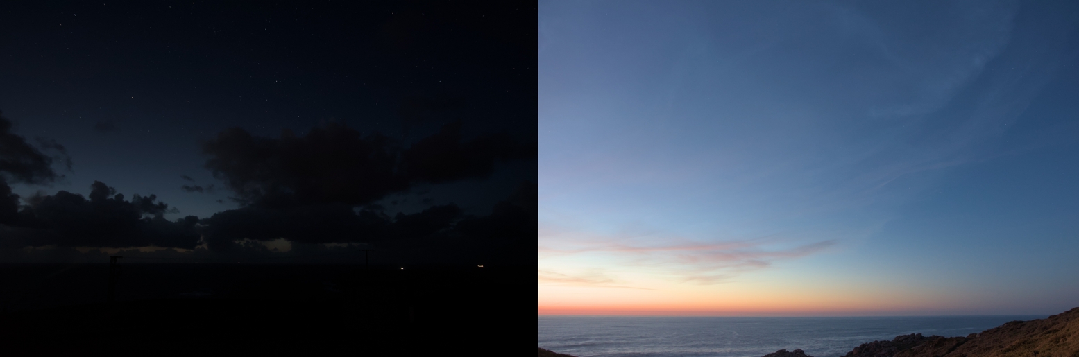
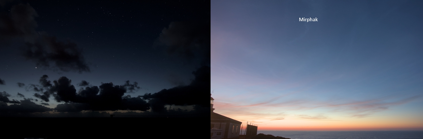
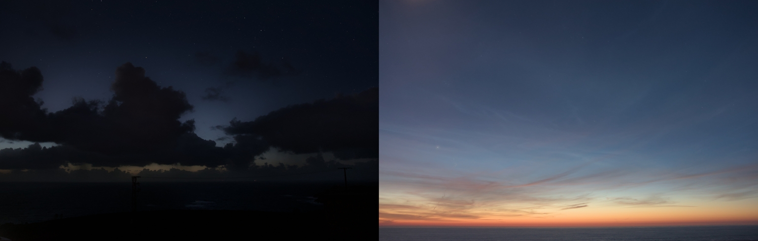
Since the solar eclipse is shallow enough, with a magnitude of at least 0.25, the limb darkening effect has the opposite consequences. In account of long wavelengths, short wavelengths are enhanced by about 2,5%. For near-horizon solar altitudes or twilight conditions, it would mean a slightly larger contribution from short wavelengths. The contribution of longer wavelengths adds a reddish tinge to the blue zenith sky in normal conditions, when the Sun is at the horizon. Contrary to popular belief, that the longer wavelengths prevail at this moment of the day, making the sky appear orange or even red, the sky at higher angular altitudes is still blue. The blue colour is modified by the reddish tinge as shown in this article. This reddish tinge is reduced when the opposite effect of limb darkening takes place. Since it’s not visible in the sky directly illuminated by the Sun, an observer can notice the relatively weak appearance of the Belt of Venus when the eclipse magnitude is smaller than 0.45. Conversely, as the eclipse magnitude increases, the Belt of Venus is enhanced as shown on webcam-based observations made a few years ago. Usually, the Belt of Venus tends to look pinkish at the lowest solar depression, but its effect weakens as the Sun goes further below the horizon. So far, only a brief explanation has been provided in this article, but it will be expanded upon in the future. The reddish tinge of the belt of Venus comes from sunlight passing through the thickest part of the atmosphere, as the Sun shines at the horizon. The aforementioned tinge is haze- and humidity-dependent, as it primarily reflects the properties of the troposphere. Considering any human activities during the day that contribute to the increase in tropospheric haze density, a more intense reddish tint is usually observed after sunset.  This brief explanation should suffice for the eclipse-induced situation in Spain, where the Belt of Venus was less pronounced. The panoramic image below shows the twilight wedge appearance (Pic. 23,24), which seems to look fainter than usual.

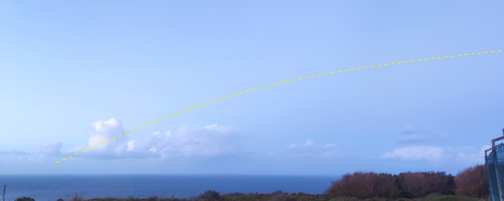
The belt of Venus at this stage of dusk isn’t pinkish, as observed shortly after sunset. Usually, it resembles a whitish band dividing the directly sunlit area of sky from the section shadowed by the Earth. In this particular moment, when the partial solar eclipse occurs below the horizon, the coloration of the twilight wedge varies in range of reddish-pinkish tinges through whitish or eventually bluish coloration. Everything depends on the eclipse magnitude and its correspondence with the limb darkening effect explained above. I was fortunate to capture the Belt of Venus shortly before the limb darkening effect was somewhat nullified at a magnitude of 0.45, which occurred only 2 minutes later after these images were taken. That’s why no difference is seen against the exact position of the Belt of Venus at normal dusk. However, on August 12, 2026, there are a multitude of opportunities to observe the Belt of Venus affected by the partial solar eclipse under various magnitudes along the path of totality. I hope this kind of observation won’t be missed as the totality occurs earlier above the horizon, giving anyone the time for “turning their heads” in the opposite direction.  Next, these observations would require repetition under similar weather circumstances. The same requirement would apply to any other circumstances in which the eclipse-induced twilight sky is observed.
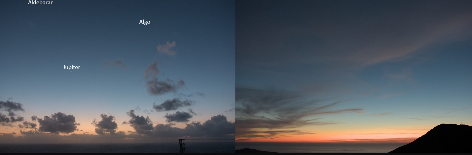
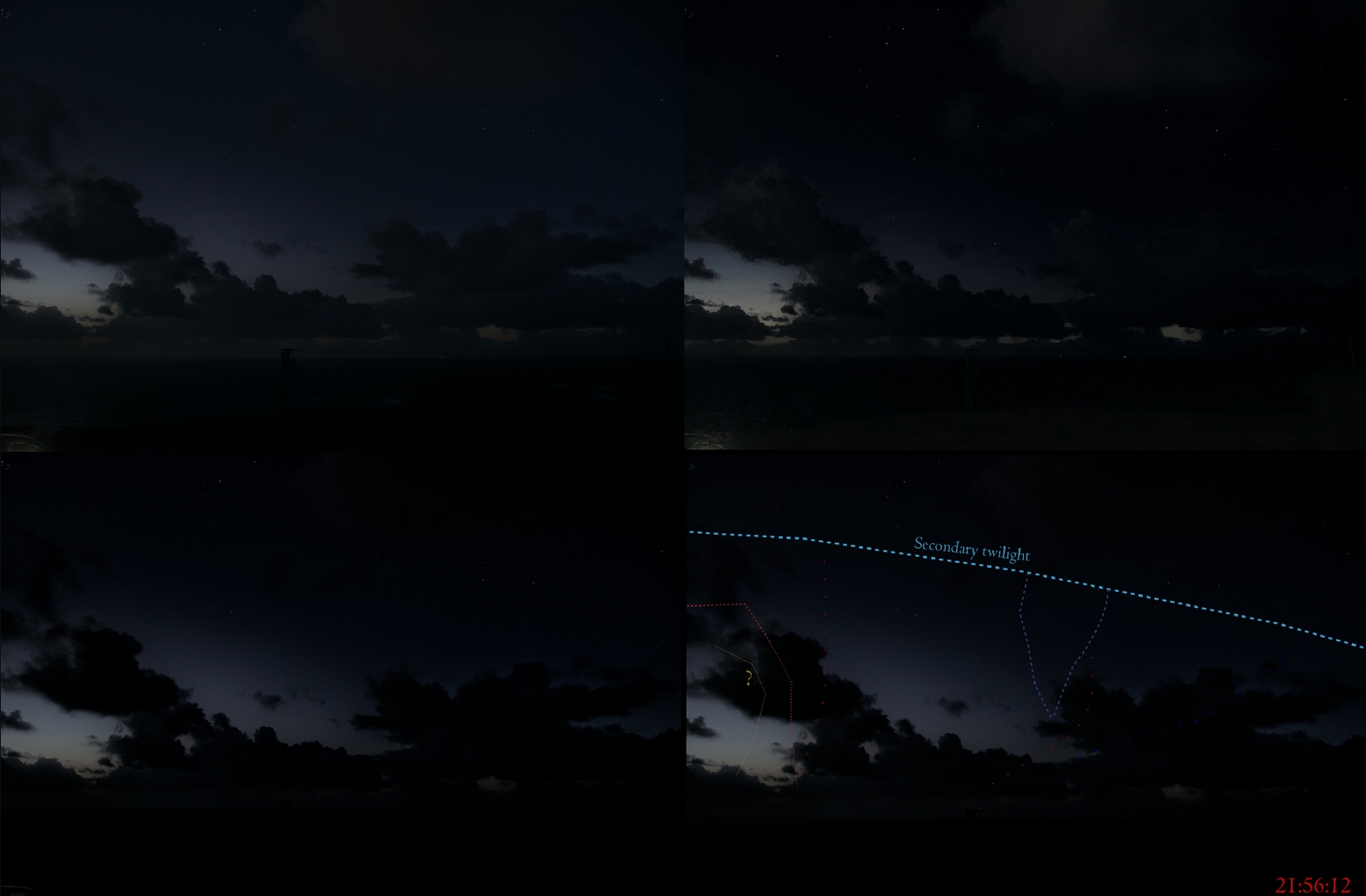
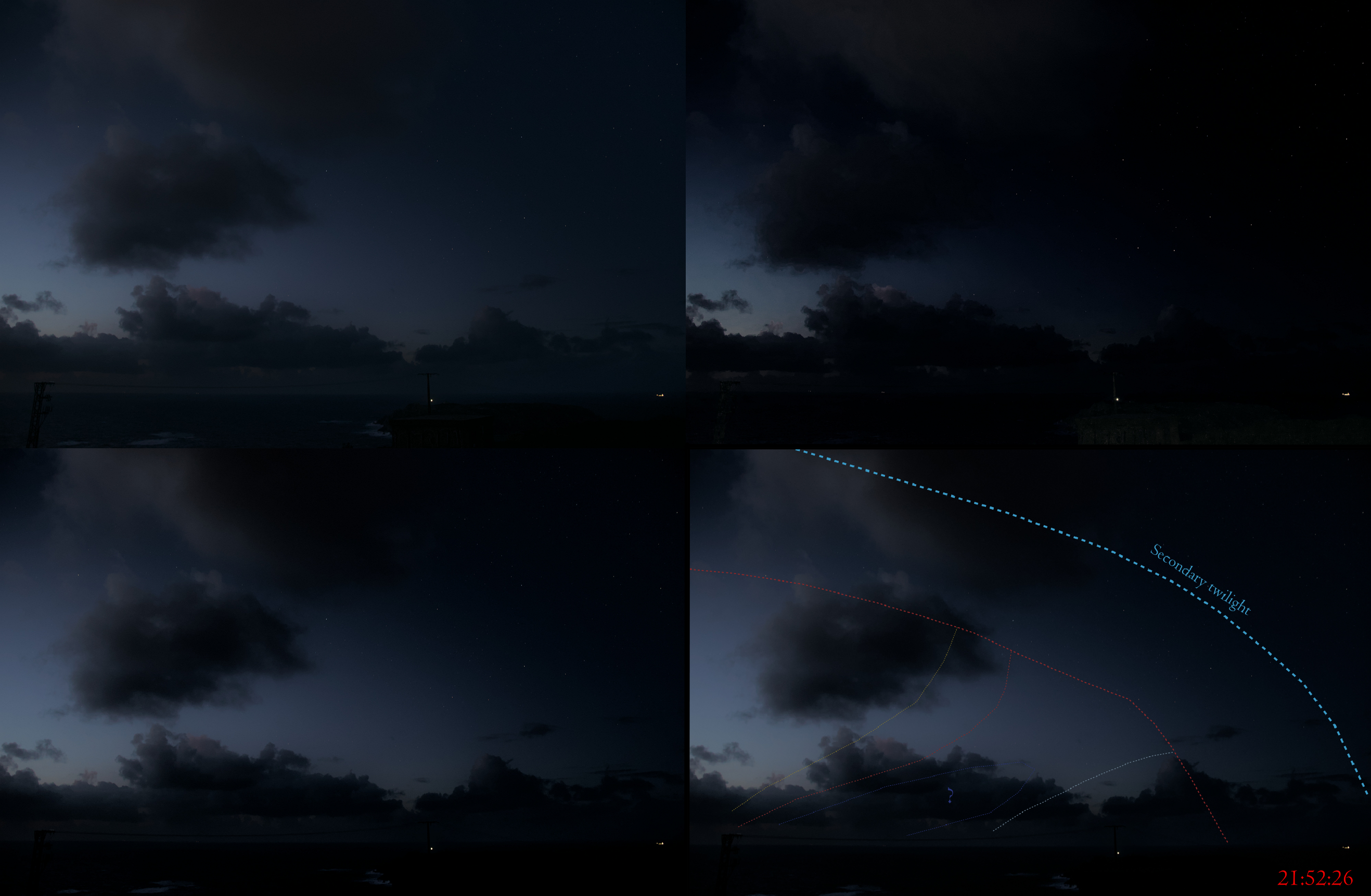
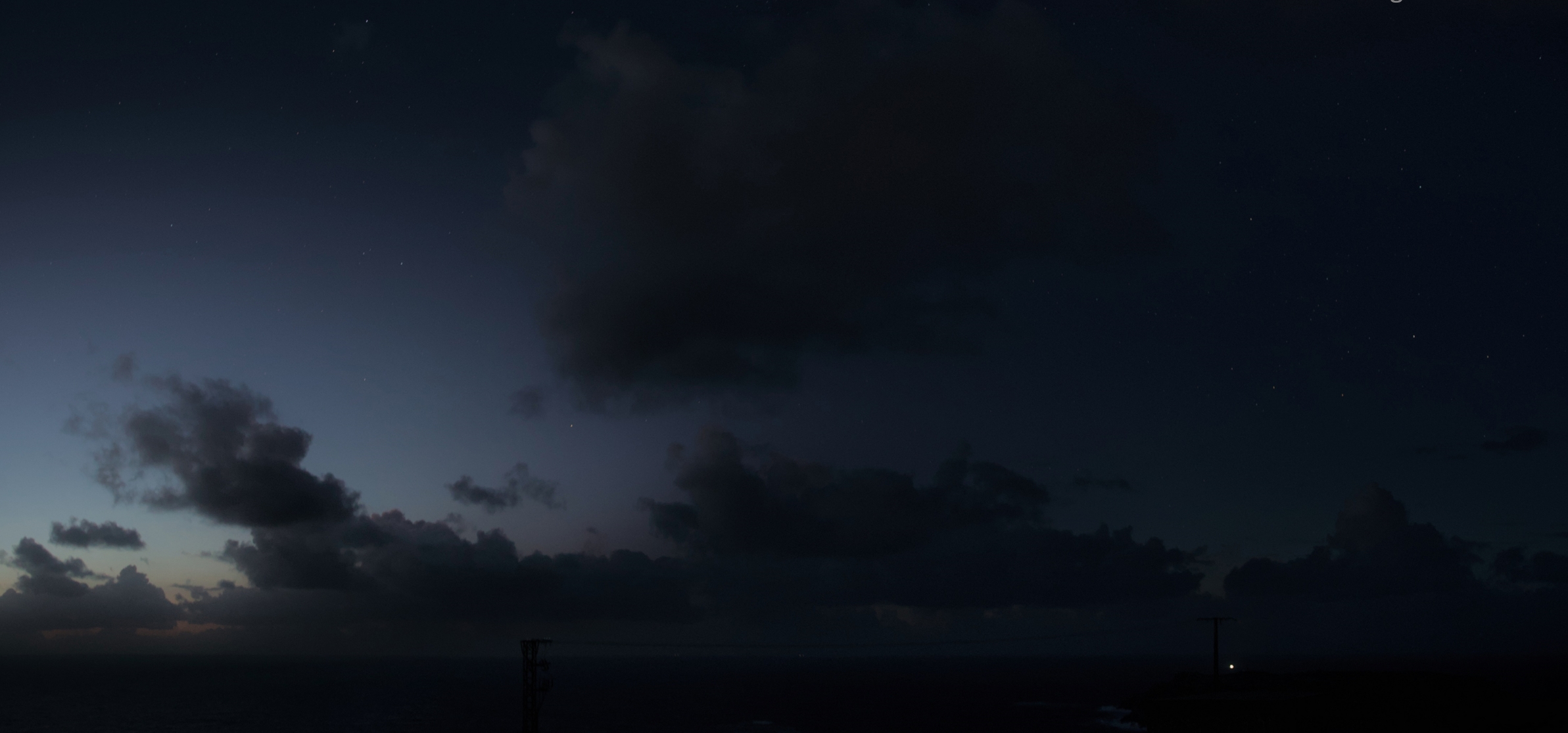
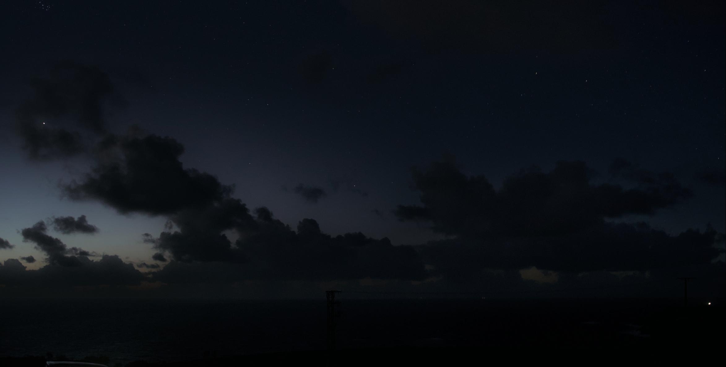
The progression of the solar eclipse, combined with the advancement of dusk, resulted in the overall Rayleigh scattering disturbance observed in the sky. The Rayleigh scattering does not seem to be a simple thing, especially at a near-horizontal viewing perspective. Apart from aerosol absorption and scattering, which occur in every circumstance, we should consider the long atmospheric path (Sundberg, 2024) of sunlight before it reaches the sky near antitwilight arch and within the secondary twilight zone. Things happen dynamically as the solar depression increases. They’re most noticeable during civil twilight, considering the antisolar direction. An observer can effectively see several different antitwilight colors, featuring dynamic solar depression-related distributions over the sky (Pic. 25).

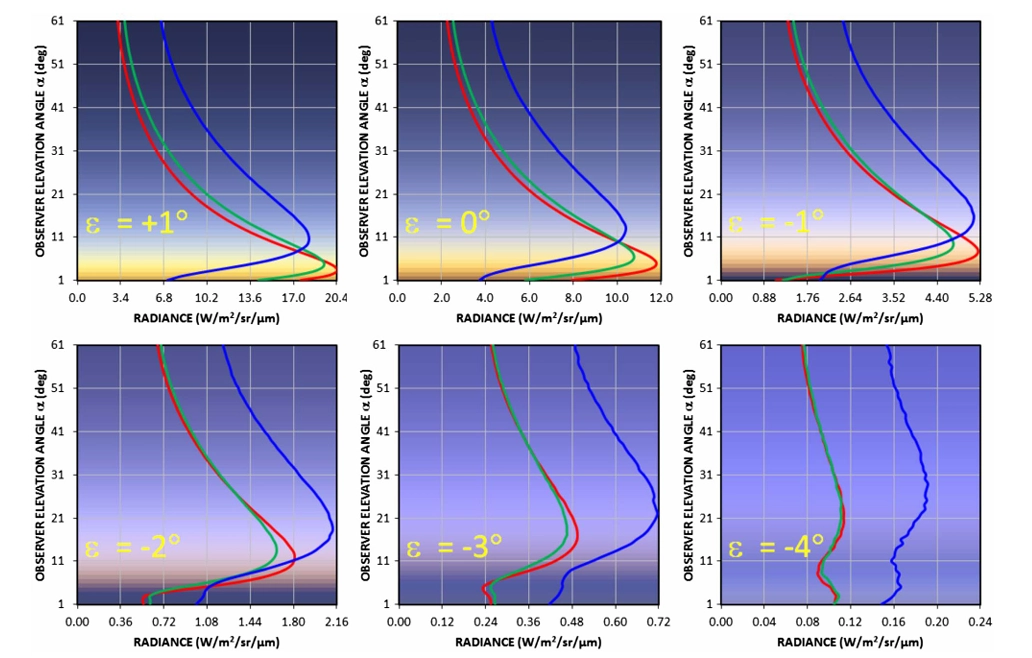
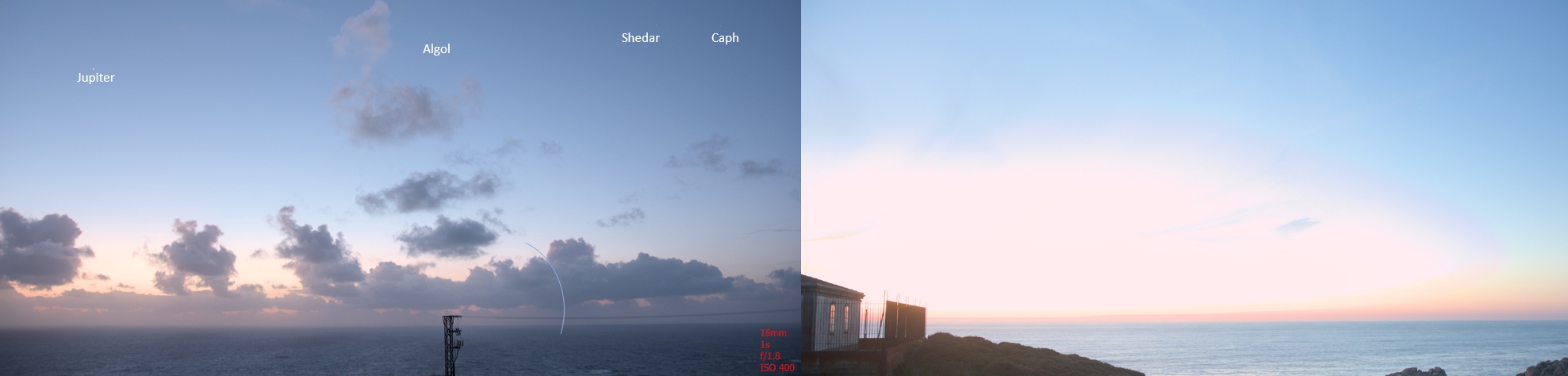
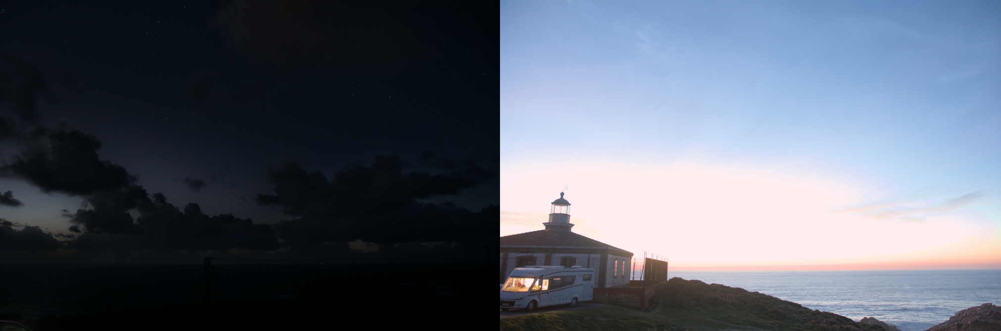
Considering the deepest part of civil twilight, for solar depression larger than 4 (ε > -4°), which was captured on April 8 in Spain, the observer is unable to see the Belt of Venus. The phenomenon fades out around a solar depression of 4°, leaving the bright band of antitwilight arch, which encloses the primary twilight section of sky. By examining the patterns above (Richtsmeier et al., 2017), we will consider the solar depression of 4° as the limit of visibility for the Belt of Venus. Beyond that, the blue hour begins, because the blue band of scattered light becomes omnipresent. The images below show the beginning of blue hour from two perspectives, where one of them is eclipse-affected (Pic. 26).

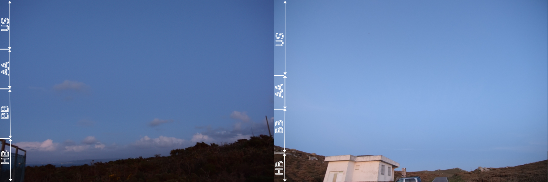
The following sections of the antitwilight sky (Ritchsmeier et al., 2017) represent various lightning circumstances at an altitude of approximately 40 km above the ground, about which some scant information can be found here and here. The upper sky (US) represents a gradual increment of the blue sky brightness, as we recognize from daylight conditions, when the Sun is high above the horizon. The sky appears bluer near the zenith, where the atmosphere is thinnest. As the observation angle decreases, the upper sky tends to be bluer, which is expressed in the brightening of the blue hue. This is because we are looking through a thicker atmosphere, which leads to an increase in sunlight extinction by Rayleigh scattering. Because the extinction cross section is significantly greater at shorter wavelengths (Ritchsmeier et al., 2017), the peak in blue radiance usually occurs right above the Antitwilight Arch (AA or ATA), resulting in a whitish sky as all the color bands overlap each other. The antitwilight arch (AA or ATA) marks the sunset visible from an altitude of 40km and therefore the boundary between the primary and secondary twilight. This transition zone is different in width as the solar depression changes (Lynch et al., 2017). The blue band (BB) is the section of sky located within the Earth’s shadow. It’s produced by diffuse sky radiation, resulting from scattered sunlight coming from the illuminated part of the atmosphere. The best appearance of blue band (BB) happens to occur where there is a local maximum in the blue channel radiance profile and the local minima in the red and green channel profiles (Ritschmeier et al., 2017). The lowest section, right above the horizon, is called the horizontal band (HB), which is significantly brighter than the blue band (BB) above. Its brightness is shaped by the presence of tropospheric haze and its ability to dissipate indirect sunlight scattered within the primary twilight zone.  Assuming that the partial solar eclipse occurs around this moment, as it did in northwestern Spain on April 8, 2024, the only visual disturbance of these colours is produced by the limb darkening effect. However, no proper example is shown in the images provided (Pic. 26, 27), as they were taken too close to the eclipse magnitude of 0.45, which, by definition, renders the effect null. Eventually, the redder direct sunlight will produce redder features in the antisolar direction (Lee, Mollner, 2017). We can’t forget about the presence of the haze. The antitwilight sky colours are the purest when the density of aerosols is the lowest, allowing purely molecular and multiple scattering to occur. However, it doesn’t work in a maritime climate, such as the one in which Galicia is located, unlike solar direction, where the most vivid twilight colors require at least some turbidity (Lee & Mollner, 2017). The limb darkening effect disturbs all these twilight chromacities.

When examining solar direction, we can observe how the color of the twilight sky gradates along the solar azimuth, from blue at the zenith to red near the horizon (Saito, Iwabuchi, & Hayasaka, 2013). From a ground observer’s perspective, the zenith sky at twilight is strongly affected by the Chappuis band, an absorption band of ozone with a peak wavelength of about 550 to 600nm corresponding to yellow and orange color (Saito, Iwabuchi, Hayasaka, 2013). When solar radiation passes a long distance through the stratosphere during twilight, the absorption at the Chappuis band makes the skylight bluer (Adams et al. 1974). Not to mention, stratospheric aerosols also contribute to the appearance of the twilight sky.

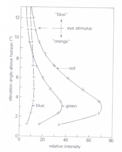
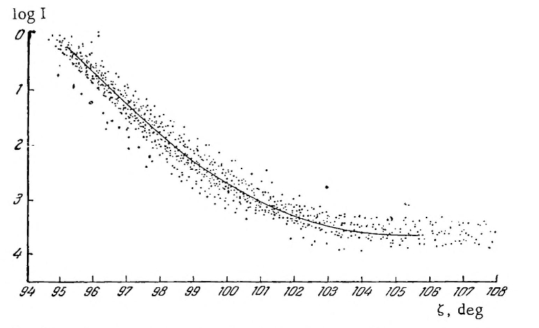
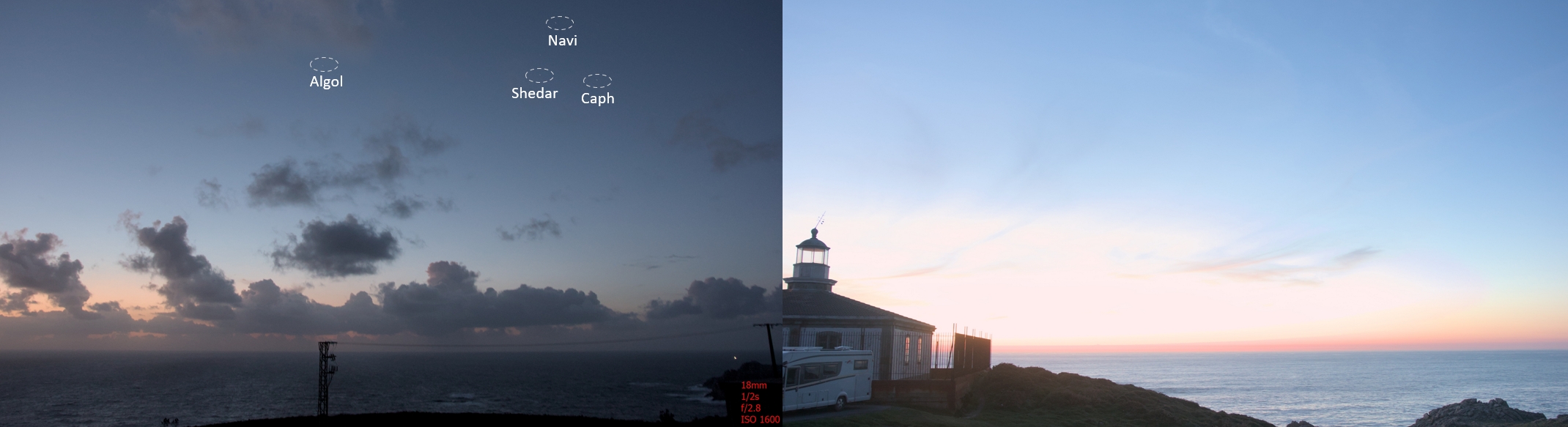
The high density of stratospheric and tropospheric aerosols makes the twilight sky redder at zenith (Lee, Meyer, Hoeppe, 2011). The richest information about the tropospheric haze is contained in the near-horizon twilight sky, where the light passes through the troposphere the longest and is expressed in the appearance of the twilight glow, which varies across different types of climates and weather patterns. For instance, the higher the humidity, the more pronounced are the orange-reddish colours during sunset (Haber, Magnol, Seider, 2005) and afterwards, when the twilight glow remains visible. The redder solar-sky colors can also be produced by increasing surface pressure and thus molecular number density (Lee, Mollner, 2017). These reddest colors are confined to a very narrow, slightly purplish band just above the horizon (Lee, Mollner, 2017). There is some accuracy to the notion that the lack of antisolar vividness results in the sky’s solar colors being more saturated with orange (Lee & Mollner, 2017). The solar half of the twilight sky features in twilight glow, which is the brightest part of the sky, a couple of degrees above the horizon. This is because light extinction occurs in tropospheric haze, especially within the planetary boundary layer. The chart on the left shows the breakdown of twilight glow by color, where the red band causes the largest horizon brightening, whereas almost no horizon brightening is reported for the blue band. The contribution of the blue band to horizon brightening is even more minor when the limb darkening effect takes place (Pic. 28, 29).

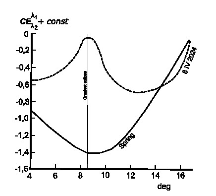
The limb darkening effect increases along with the eclipse magnitude, since it’s higher than 0.45. The upper sky, being a subject of Chappuis absorption, is an increasingly mixed blend of dark blue and reddish hues. The blue colour results primarily from ozone absorption rather than molecular scattering (Lee, Meyer, & Hoeppe, 2011), which appears to be even more intense as the ozone layer builds up during the eclipse (Zhang et al., 2025). Because the Chappuis absorption, along with Rayleigh scattering, contributes to the blue color of the sky, the limb darkening effect is noticeable in slight reddening. Another matter is the wavelength breakdown proportion of sunlight modified by limb darkening, which is most pronounced at the shortest wavelengths, unlike the Chappuis absorption, which affects longer wavelengths. Therefore, the reddening of the twilight sky is apparent and changes with its proportion due to variations in solar depression, shaping the spectral composition of the light. The reddening of the sky is an intrinsic phenomenon of the golden hour and twilight, which gradually diminishes to the moment of deep civil twilight due to the blueness of the sky. Next, it increases again from mid-nautical twilight. It reaches its maximum level at the deepest phase of astronomical twilight, as determined by the color index considered for the zenith sky (Rozenberg, 1966). The evening of April 8, 2024, was specific as the twilight was affected by a deep partial solar eclipse. Hence, the sky reddening pattern had presumably the inverted shape, concluded from visual observation that evening (Pic. 28), which is assumed to reflect the influence of limb darkening over the eclipsed twilight period. Detailed estimation will be required in future observations, computations, and measurements, although for the time being, a good hint is provided.

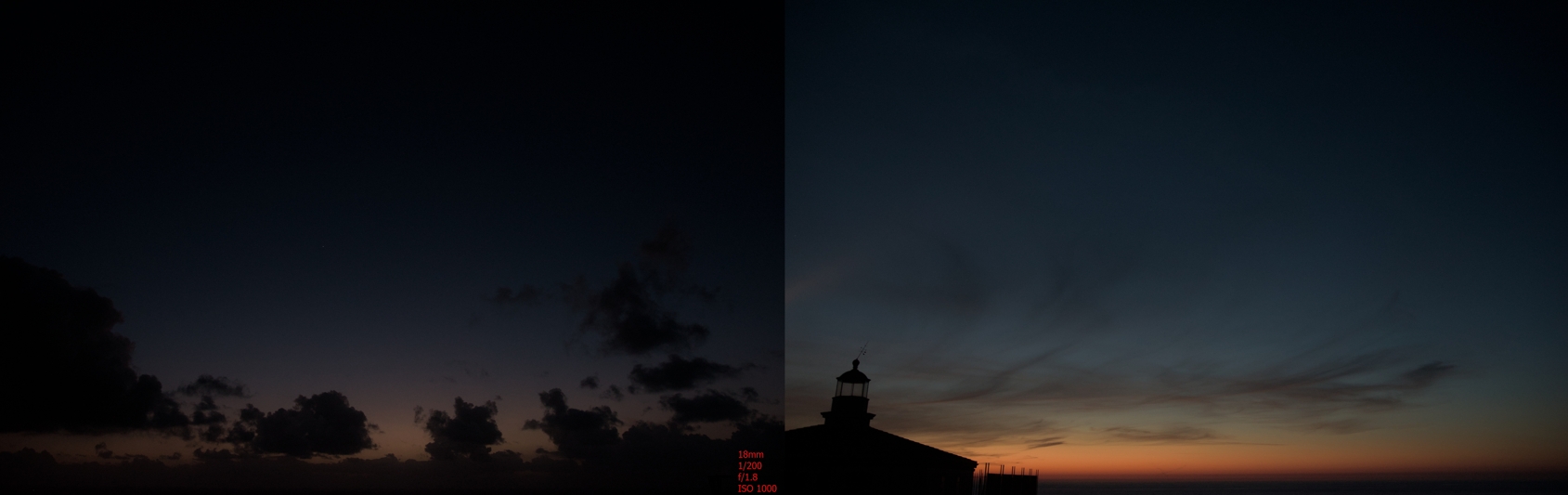
The influence of the solar eclipse on the twilight sky is expressed nicely at shorter exposures, which don’t allow much light to get in. Apart from the noticeable changes in sky illumination, considered later in this article, the eclipse-induced reddening of the sky is more visible across the entire twilight sky profile. The sky reddening is a subject of seasonal or even diurnal variations, depending on the weather conditions, mainly the level of moisture and density of tropospheric haze. The increment of sky reddening, particularly at zenith from mid-nautical twilight onwards, has a similar result to near-sunset conditions observed from the ground, when longer wavelengths pass through a thick atmosphere. The effect from the stratospheric position can be better, as the thickest atmosphere is visible edge-on against the blackness of space.

The beginning of nautical twilight shows the different position of the red segment of the sky. In normal twilight conditions, an observer can see the afterglow resulting from direct sunlight scattering at the lowest part of the atmosphere, which, from a geometrical point of view, lies closest to the terminator line. The yellow-orange-pinkish tinge is an effect of sunlight extinction in the thickest part of the atmosphere observed from a stratospheric position. The eclipse-induced beginning of nautical twilight represents the same pattern, but the red segment is observed just above the afterglow zone. This is the effect of the relatively high color index ratio discussed above. At lower altitudes, such as this, the Chappuis absorption has a minimal influence.

This trend continues over the eclipse’s progress during nautical twilight up to its greatest phase. At maximum, an observer could see the pinkish band located at the boundary between the primary and secondary twilight. This is because the limb darkening effect is strong enough to produce the optical outcome seen in this case.

The greatest eclipse occurred shortly before the mid-nautical twilight. Technically, the period of nautical twilight means that the directly illuminated section of sky gradually yields to the sky located within the Earth’s shadow. In civil twilight conditions, it’s defined as the dark segment or twilight wedge. However, the twilight wedge marks the boundary between the primary and secondary twilight in the nautical zone, too. From a geometrical point of view, the boundary between the civil and nautical twilight is marked by the zenithal position of the twilight wedge and its angular distance of 90 degrees from the solar azimuth in any direction. Hence, the nautical twilight shall be understood as the period during which the twilight wedge is located only within the solar half of the sky, being enclosed within at most 180 degrees of angular span. As nautical twilight progresses, this twilight wedge moves further towards the solar azimuth and becomes visible at a lower elevation in the solar half of the sky. However, due to the still strong scattering of the twilight glow, it is not pronounced well. Despite the multitude of explanations of the twilight wedge as the zone of sky shadowed by the Earth, some sources explain the phenomenon as the fairly sharp boundary between the illuminated sky and the shadowed sky, which is correct. However, the phenomenon is considered only for the early stage of civil twilight, with its position in an antitwilight sky. In contrast, it can be visible until the deepest phase of nautical twilight.
From the observer’s point of view, on the evening of April 8, 2024, the appearance of the twilight wedge resembled somewhat the Belt of Venus. Typically, there is a quite sharp transition, which, due to the Chappuis band, shows the blue band. The twilight wedge, which represents the sunset at an altitude corresponding to the ozone layer, receives analog optical components of sunlight as we know from the near-sunset conditions on the ground, where, due to Rayleigh scattering, the short wavelengths like blue are scattered away, and longer wavelengths in the spectrum from yellow to red pass through the thick atmosphere. The atmosphere from an altitude of about 40km looks different, as it’s compressed and visible edge-on against the blackness of space. Unlike the ground-based sunset, the sunset at the stratosphere appears different, as only part of the solar disk is affected by the thick atmosphere (Pic. 33), thereby making the Rayleigh scattering behavior more complex.

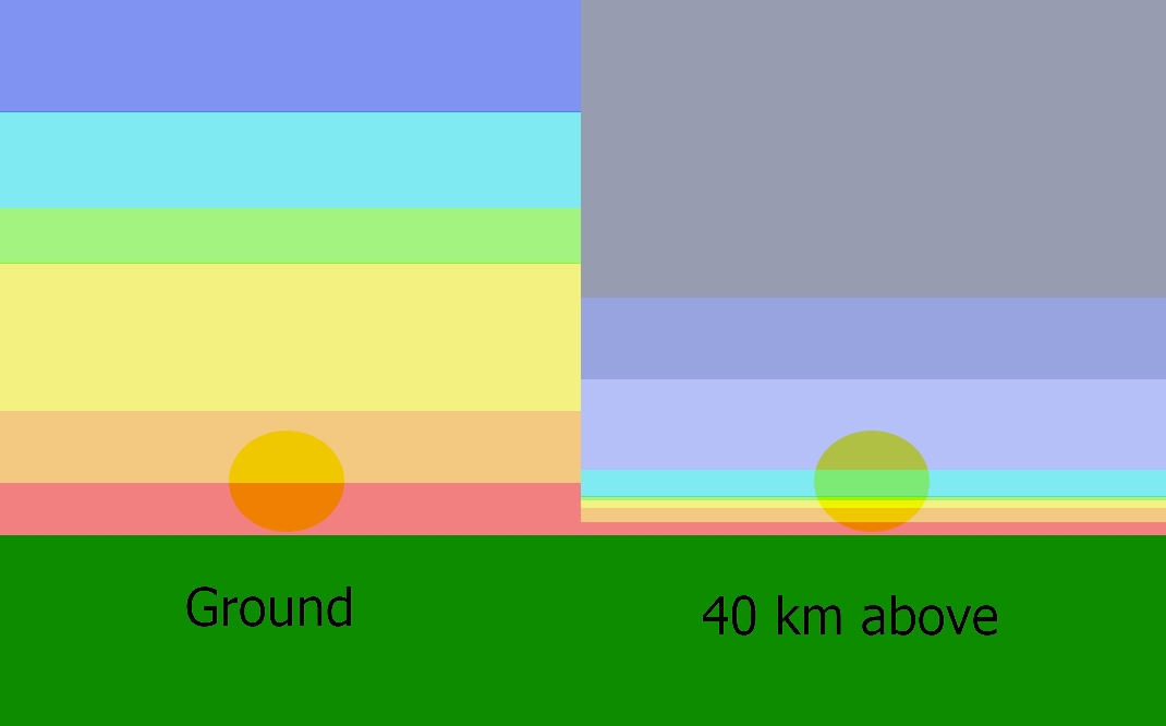
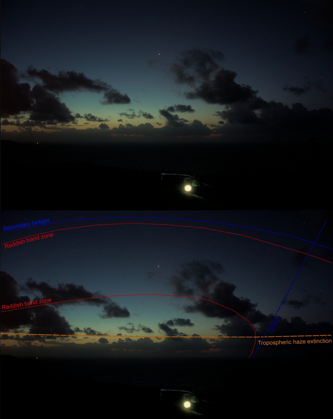
Since the sunlight from the lower part of the solar disk looks reddish, the sunlight coming from the upper part of the solar disk will remain the same throughout the day. The outcome of sunlight coloration under these circumstances is presumed to be yellow. Because of the strong effect of Chappuis absorption in reducing the intensity of some of the rays, the color changes from yellow to blue or blue-purple (Hulburt, 1953). As the Sun plunges beneath the horizon, the contribution of longer wavelengths increases, but the amount of sunlight decreases simultaneously. It leads to understanding the specificity of the twilight wedge, which, for the sake of simplification, can be characterized as the increment of long wavelengths inversely proportional to the amount of sunlight. Since only the upper edge of the Sun is visible above the elevated horizon, the amount of light is too small to contribute seriously to the overall color of the sky. In turn, this sharp band in the sky remains mostly bluish. Things become different as limb darkening comes into play. During a deep partial solar eclipse, the proportion of light wavelengths within the twilight wedge is significantly modified by a substantial contribution from red wavelengths, resulting in a corresponding reddish band. Eventually, the sky coloration in this particular zone appears to have a pale green tinge, which is an effect of Chappuis absorption, which peaks at a wavelength of 603 nm, thereby eliminating the contribution of yellow coloration. The spectroscopy of the twilight wedge appears dynamic, as the pale green sky gradually transitions into blue as it moves into the primary twilight zone. This twiligh twedge tends to change its optical specificity when moving closer to the umbral zone. This is because the increasing eclipse obscuration triggers a more intensive influence of the limb darkening phenomenon. This is why the reddish band zone, which is visible above (Pic. 32), tends to be wider and slightly more intensive, even darker towards the right. The most noticeable spherical difference of limb darkening contribution is visible in the direct vicinity of the extended path of totality.
The sky looks interesting, especially within the section shadowed by the Moon. Shortly after the umbra leaves the lower atmosphere, the intensive reddish influence can be noticed in the direct vicinity, which is the result of the greatest effect of limb darkening. The image sequence below shows how the effect weakens quickly as the umbra moves away from the atmosphere (Pic. 34).

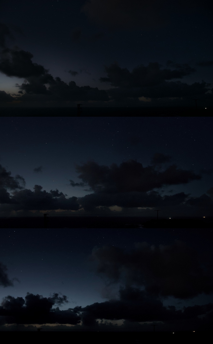
The uppermost image represents the third contact in the stratosphere. The twilight glow appears very dim, with an omnipresence of reddish coloration, which shifts towards pale green as one moves further from the path extension. The middle image was taken 2 minutes later and still shows a significant impact of lib darkening, where the entire twilight wedge features the pale greenish band zone caused by the factors discussed above. The last, bottom image shows the twilight wedge, which is the closest to customary conditions, as the pale greenish band gradually turns into blue.
The following sequences couldn’t be obtained correctly due to increasing cloudiness and passing rainfalls visible near the horizon (Pic. 35,36). These meteorological obstructions blocked the visibility of the twilight wedge.

The only rational conclusion visible in these images is the different specificity of the twilight wedge, which is affected by the eclipse. Since, in normal conditions, it appears as a fair blue band that is not discernible enough from the twilight glow underneath, the eclipse-induced twilight wedge represents a sharp transition between the primary and secondary twilight, with an intensive, although systematically decreasing, pale green tinge.

5. SKY SURFACE AND OVERALL BRIGHTNESS CHANGES

The influence of a solar eclipse on twilight results in changes in the sky’s surface brightness and the overall brightness of the scene. Indeed, these changes are most noticeable, especially when the eclipse magnitude is large enough. Getting dark is the most trivial thing, which can be detected by most of us as a consequence of the progressing eclipse. Based on the approach of amateur observation carried out in 2017, supplemented by external data from Wolfgang Strickling, a well-equipped German eclipse chaser, the sky surface brightness is not distributed uniformly during the eclipse. Furthermore, the various distributions are typical primarily for non-eclipse conditions unless the Sun shines near zenith.

Otherwise, the brightest section of the sky is located near the solar azimuth. It looks analogous to the light scattering on aerosols and haze under daylight conditions. If this is the case, the presence of the solar eclipse complicates the problem in question. However, during twilight conditions, the situation is different. First, direct sunlight scattering on aerosols and haze doesn’t occur unless we consider civil twilight. Civil twilight means that there is at least a small section of sky in which the sunlight is scattered directly on tropospheric haze. This is the section of the solar half of the sky, and even so, this kind of scattering has a tiny contribution compared to daylight conditions, regardless of the stage of civil twilight. As we know from the previous chapter, the twilight sky is specific, because it changes dynamically, especially at the most minor solar depression. Eventually, the twilight sky represents two major bands separated by the hypothetical terminator line in the stratosphere at an altitude of approximately 40km. It adds another complicated factor for understanding the sky surface brightness. For this purpose, the twilight sky is considered moonless and utterly free of light pollution. Additionally, the presence of tropospheric haze may also make a significant contribution to the overall brightness of the twilight sky. When the sky is more humid or the density of aerosols is high, then the scattered sunlight extinction will be higher, making the twilight slightly darker as usual (Pic. 37).  Finally, the twilight glow depend markedly on wavelength and because of atmospheric extinction, the maximum brightness doesn’t occur at very horizon, but a bit higher. Considering the typical situation, in which the twilight proceeds normally, the distribution of brightness observed at the solar part of the twilight sky is symmetrical to solar azimuth regardless of the solar depression (Pic. 38).

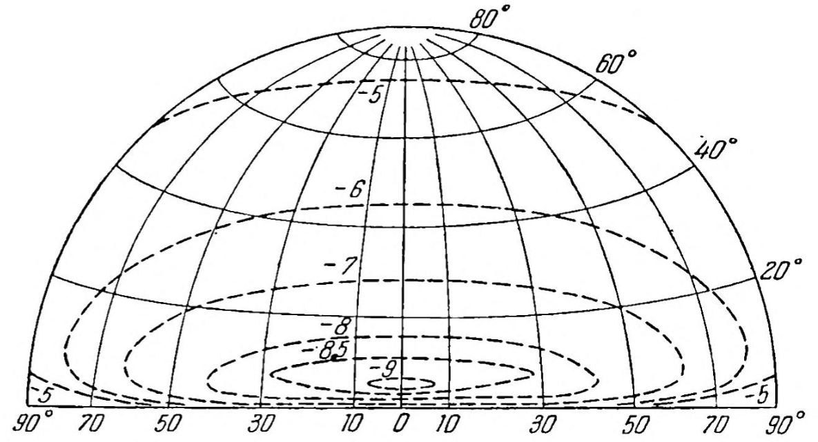
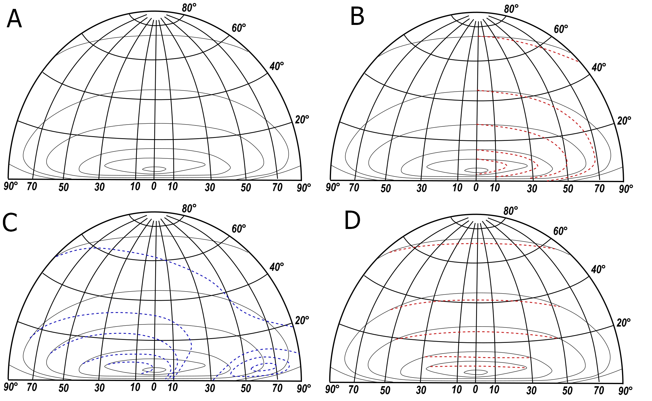
The image on the right shows the brightness of the twilight sky at solar azimuth at the brightest part of civil twilight, with all labeled isophotes. All these isophotes are symmetrical to the local azimuth of 0, indicating roughly the position of the Sun beneath the horizon. It doesn’t occur this way when the eclipse takes place, but there are some cases in which this pattern can be almost the same even if the eclipse occurs. Because this thread requires a separate study, I want to list the few situations where these isophotes will have other shapes:
A: the greatest magnitude of the partial eclipse, or extension of annular eclipse observed at the location,
B: the extension of the annular solar eclipse path at the location,
C: the extension of the total solar eclipse path at the location,
D: the sideline view of the total solar eclipse extension from the location,
E: the sideline view of annular solar eclipse extension or partial solar eclipse influence on twilight away from the greatest phase at the location.
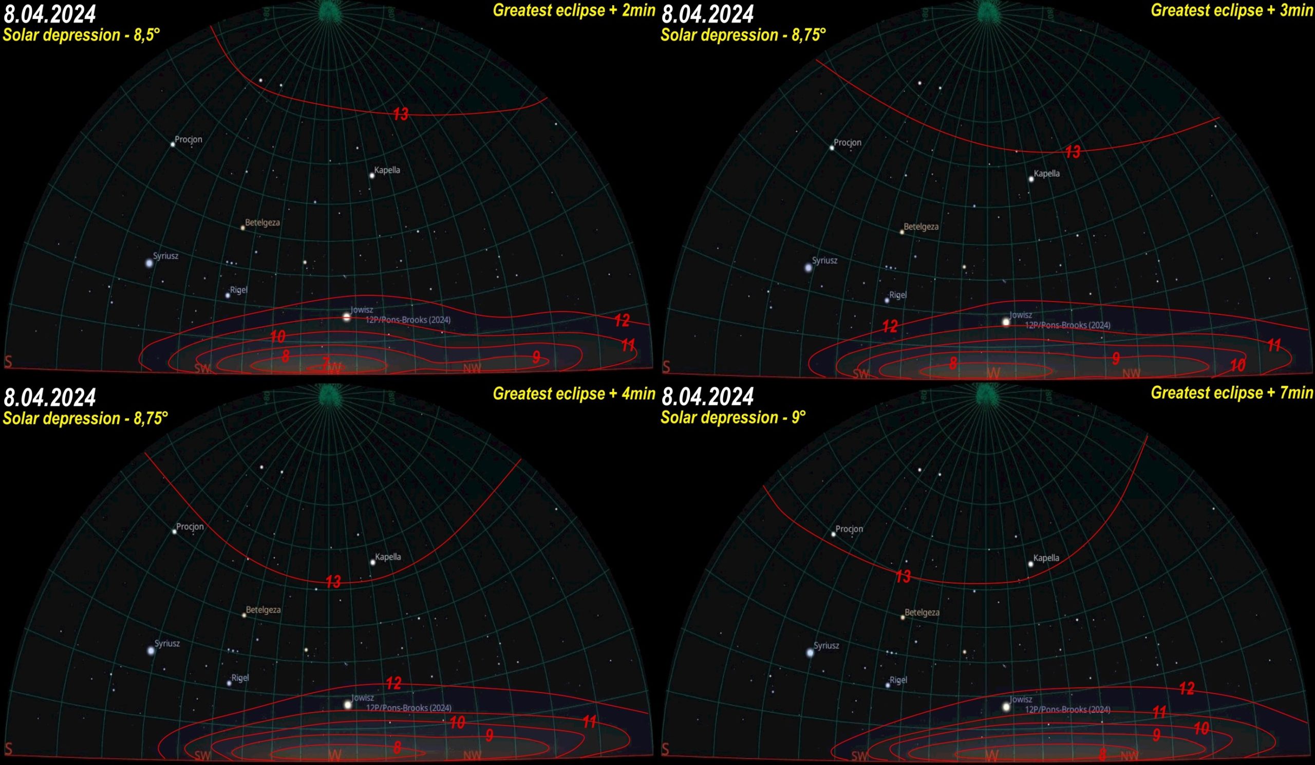
The situation from April 8, 2024, applies to points D, E, and A because there was no total solar eclipse at the location, and only the deep partial phase was observed. In this case, an observer experienced at most the sideline view of a total solar eclipse around its greatest phase. Before and after this moment, the twilight was affected by the partial solar eclipse, not at its maximum greatest phase. In a practical sense, these two cases fit perfectly with the potential isophotes asymmetry, which has been considered using Stellarium 25.2 and GIMP 3.0.4 software for four moments of the April 8, 2024, solar eclipse’s impact on twilight in Spain (Pic. 39).

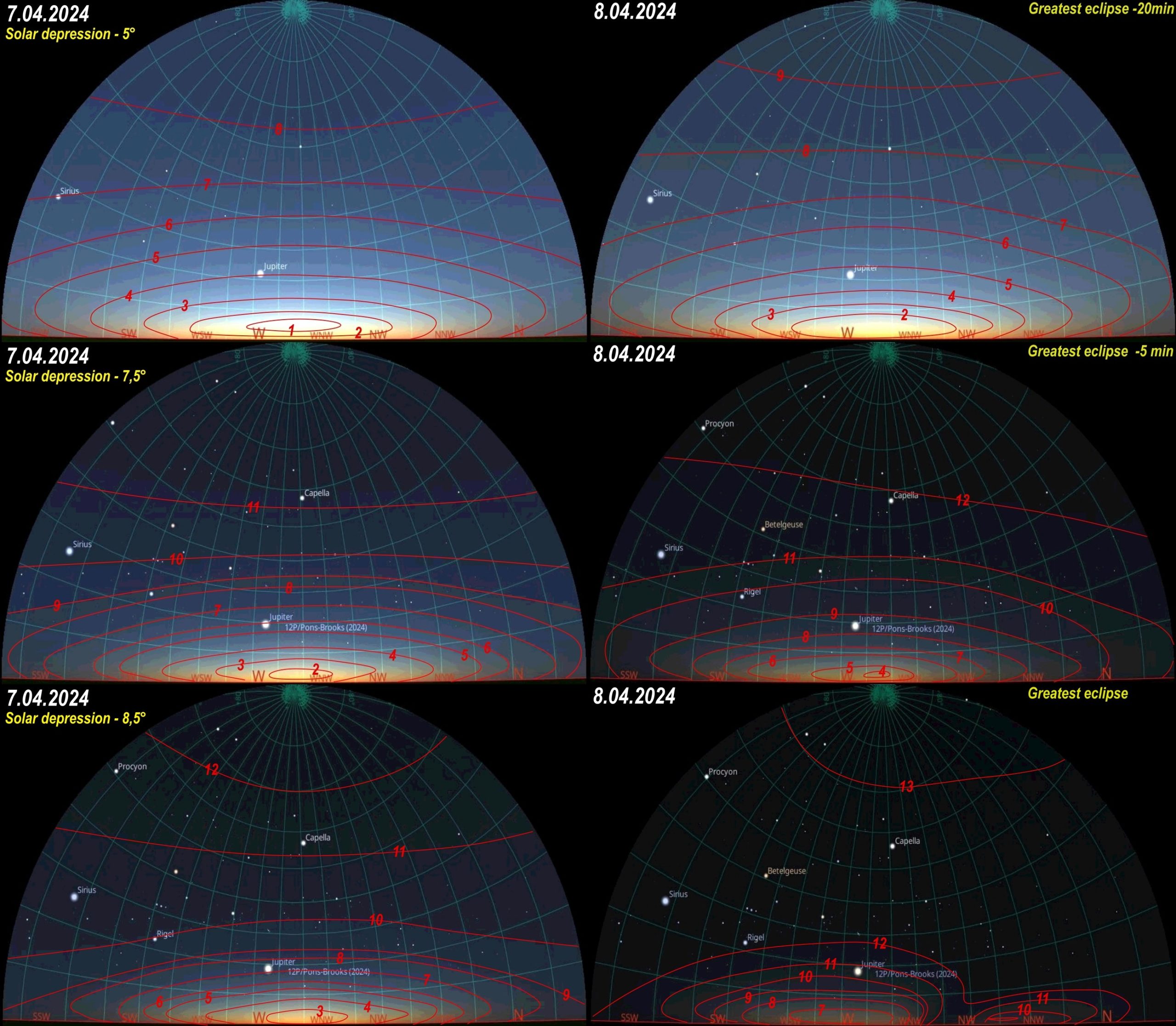
Assuming the base twilight brightness represents the base twilight brightness, we can see the sky surface brightness classified between 1 and 8, where the number 1 refers to the brightest part of a narrow section of the sky just above the horizon, approximately at the solar azimuth. The solar depression of 5° means deep civil twilight, but within the section bounded in 1 we can still see the high level clouds illuminated by the setting sun. This is a way of considering these points, but it would give you a hint of what bright this isophote defines in the sky. Next, we see progressively darker sky as the angular distance from solar azimuth increases. The darkest part of the sky is near the zenith, which should be understandable. By looking at the same sky on the right, where the partial solar eclipse progresses with obscuration of over 50%, a slight asymmetry becomes apparent from the north direction (right), and the sky appears slightly darker. However, further progress in the eclipse leads to a more significant asymmetry in sky surface brightness. At a solar depression of 7.5°, isophote number 11 marks the boundary between primary and secondary twilight. Under eclipse conditions with an obscuration of 85%, this boundary is narrowed and hard to detect, as isophote number 12 comes into place and its shape slants towards the north. The greatest eclipse marked umbra visibility at the northwest direction side away from the solar azimuth. The isophotes show clearly two separate sources of brightness, which correspond to the divided twilight glow. Because the greatest obscuration at the observation location was 94,2%, the effect was somewhat like the side view of a total solar eclipse. The isophote with number 12 indicates the significant disturbance at the line between the primary and secondary twilight. Beyond this line, the sky was featureless, with slight darkening towards the zenith, where the darkest isophote, number 13, still displays asymmetry. Noteworthy is the shape of isophote number 12, roughly at the intersection of the umbra and Earth’s shadow. It clearly shows that the umbra is brighter than the Earth’s shadow. More about it is presented in a later chapter. Considering the aforementioned isophote configurations, which were visible on April 8, 2024, twilight in Spain, we can present them in the following sketches below (Pic. 40).

The situation, which was observed shortly after the umbra was visible in the atmosphere, is interesting. This is the situation corresponding to a Gamma value higher than 1, when the eclipse is no longer central anywhere on Earth. The problem has recently been discussed in the context of analyzing the last partial solar eclipse, which occurred on March 29, 2025. Because the Moon changes its position against the ecliptic, its path isn’t straight. Regarding the type of node, the path can proceed northward or southward, and its relation to sunrise or sunset will have an additional, separate contribution, which is discussed in a further chapter. By now, we can be aware that once the umbra leaves the Earth’s surface and thereby the atmosphere, the eclipse still has its greatest phase somewhere outside the path. The area of the greatest phase is initially adjacent to the path extension and moves away later on. Finally, for an observer standing within the twilight zone, the isophotes might show the “flattened” shapes roughly at solar azimuth and have a twofold meaning, which can occasionally apply to the extent of the annularity path. I was only partially fortunate to see it in Spain because of the weather, which worsened later after the main eclipse spectacle. As mentioned above, this is the subject of another thread to be explained in the future. Some of you may wonder where this asymmetry comes from.

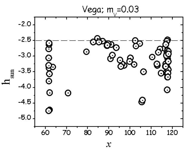
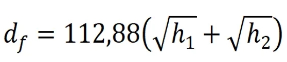The spherical assymmetry of sky surface brightness as occurs during partial solar eclipse arises out of the distance of sky sphere visible for an observer. Considering the crucial altitude of 40km discussed earlier, I could technically see the sky from a maximum distance of 758 km in all directions. This distance can be obtained from the formula on the left, which neglects refraction issues and includes an observation altitude of 150 m.s.l., where:
df – the distance to the horizon
h1 – the distance of an observer
h2 – the distance of the object observed

This formula can be written in Excel accordingly:

Df = 112,88*(SQRT(H1)+SQRT(H2))

Concluding, when an observer watches the sky in the span of 180°, theoretically, he could reach as far as 1430 km from one direction to the opposite one. In my case, it could be as far as 1514km between opposite directions against the solar azimuth. However, we must realize that these extreme distances are unrealistic to achieve from a ground perspective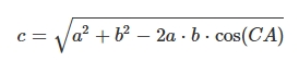 because of tropospheric haze, the potential presence of clouds, and other elements. Being more realistic, we shall narrow down this perspective to the visibility of the sky at least 3° above the horizon in any direction. For this computation, we need to consider the slant distance, which is the line of sight between two points with different elevations. The slant distance between the observation place and the place at which the considered point of sky at an angular altitude of 3° would be visible exactly at zenith. The formula can be found on the right, and its explanation is provided here.
Analyzing my situation in Spain, I could watch the sky as far as 454 km in any direction and at most 908 km in the span of 180°, excluding topographic obstacles. Anyway, this distance is pretty significant to mark the spherical difference in sky surface brightness when the eclipse occurs, as displayed in the sketch below (Pic. 41)

The sketch above roughly illustrates the question about the non-uniform distribution of sky illumination in the twilight sky, which is affected by the solar eclipse. Since the observer is standing in the bottom middle of the graph, the twilight sky is affected by the solar eclipse to some extent. However, when the same observer turns his head 90° to the left, he should see a slightly brighter portion of the sky, as the same eclipse phase at a distance of 454 km is smaller. The same thing applies to the opposite direction, where the sky is affected by the deepest phase of solar eclipse, and therefore should look darker. When the umbra is close enough, these changes become more pronounced, causing the sky to darken abruptly. Finally, the umbra’s presence makes the twilight glow divided between two separate sources of light.
The sky surface brightness is also affected by the factors adequate to typical twilight (Pic. 38), which include:
– the angular distance to the solar azimuth,
– solar depression,
– altitude above the horizon,
– degree of atmosphere clarity.
The combination of all of them leads to a complex understanding of the threshold of stellar visibility. In general, we can assume that some sort of stars are visible at the specific moment of twilight, characterized by the individual sky surface brightness conditions. The great rundown can be found in the chart below (Pic. 42), and discussed on the occasion of planning this observation.

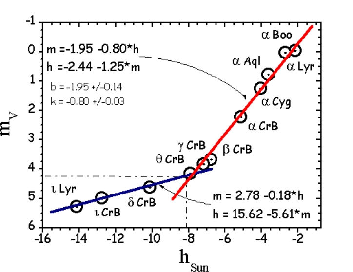
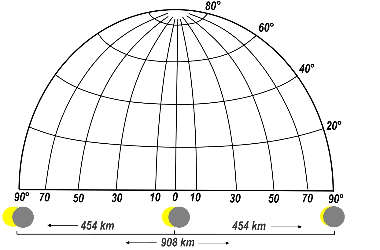
The results above apply to the situation, in which the atmosphere features a high level of clarity, although it doesn’t happen every day. When the factors discussed above are applied, the chart would look more complicated. For example, the Vega star was chosen because of its apparent brightness of nearly 0 Mag (Fig. 43).

Under extremely clear atmospheric conditions, the Vega star can be visible at solar depression lower than 2,5°. In practice, the star can be visible to the naked eye between some high-level clouds at zenith, still illuminated by the setting sun. At this moment of twilight, even mid-level clouds at solar azimuth catch the direct solar beams. Analyzing an opposite situation, Vega could become visible at a solar depression of over 4.5 ° under the least favorable conditions (Nickiforov & Belokrylov, 2011). Another consideration is the optimal moment of visibility for any celestial body within the twilight zone. It doesn’t apply to stars like Vega, because they are usually located far away from the Sun. This particular problem is typical for Mercury or some comets, whose observation conditions are generally demanding. Their long elongation angle from the Sun provides only a short period of optimal visibility to the observer, considered the “observation window” (Kastner, 1976), as shown in the graph below (Fig. 44).

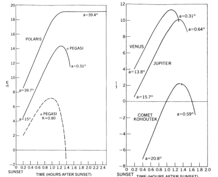
As discussed here, each object has its own “arc of visibility” featuring the best moment, when we can perform the observation. These “arcs” are different for each individual object as an angular distance-dependent thing. When the object is far away from the Sun, the so-called “arc” doesn’t exist as the object remains visible well beyond twilight. On the other hand, when an object is too close to the Sun, its visibility is restricted, making the “arc of visibility” very narrow. In contrast to the sky surface brightness at twilight, each single object has its elongation angle, beneath which it becomes invisible to the observer’s eye. This is because the Earth’s atmospheric extinction occurs and varies according to the degree of atmospheric clarity. The occurrence of a solar eclipse at twilight contributes to the general “arc of visibility,” making it eventually wider. The “observation window” is always better and lasts longer, depending on the magnitude of the eclipse at the given moment. Because it’s hard to gauge the visibility of celestial objects individually, the best approach is to estimate the general level of brightness, which works well as a matter of simplification. The one-directional measurements of sky surface brightness on the evening of April 8, 2024, prove that this method generally works in a holistic sense (Fig. 45-47).

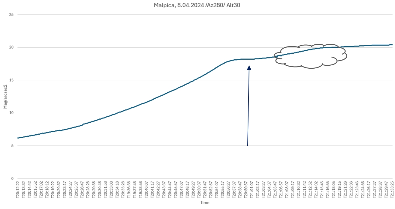
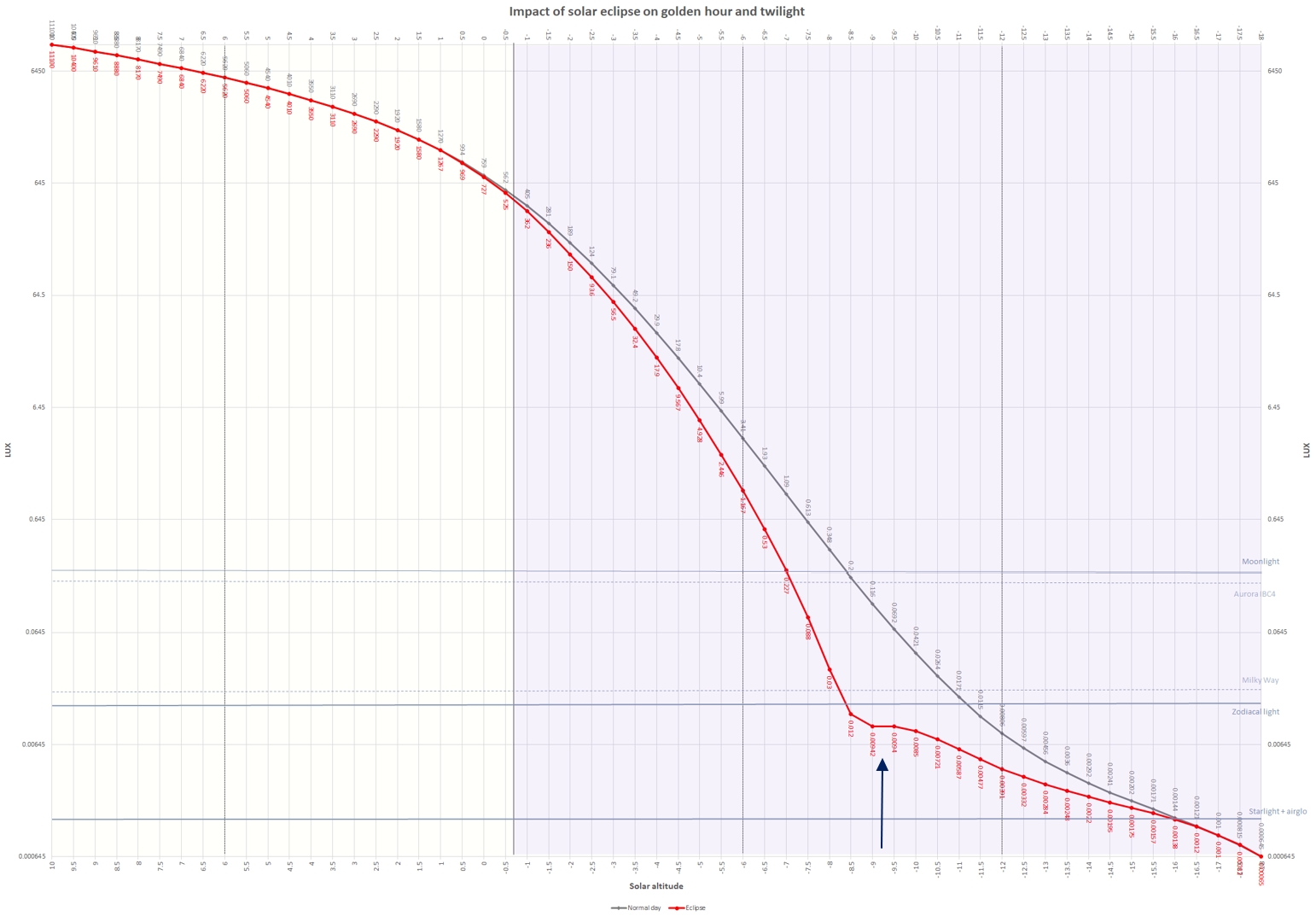
The comparison between the measurement (Fig. 46) and computation (Fig. 47) illustrates a simplified method for estimating the overall brightness at twilight during an eclipse. This approach can be applied to the sky surface brightness model as long as it’s considered uniformly, without any asymmetry in isophote distributions. The complex solution will be investigated on another occasion. The similarity between the measurement and computation comes from the common denominator considered for both, which is the approximate direction of solar azimuth. In the case of computations, the general brightness of twilight is determined by the glow located near solar azimuth, which gives proportionally the largest amount of light. Applying the calculations such as above (Pic. 47) allows us to assume what stage of typical twilight the eclipse-induced twilight corresponds to. It’s presented further in this article as an updated twilight nomograph. Analyzing the chart above (Pic. 47), an observer can gauge, that the greatest eclipse at solar depression of 8,6° resembled the very deep nautical twilight at solar depression of almost 12°. The ambiguity of this understanding lies in other directions. I can’t confirm this difference for the azimuth forther north, where the umbra appeared. There were completely different circumstances. However, as long as the eclipse phase is not large enough, this method is fine, as can be seen in the images below (Pic. 48 – 52).

The most interesting sky surface brightness circumstances occurred near the greatest eclipse phase. The images above (Pic. 50-52) and below (Pic. 53) display the sky surface brightness asymmetry visible at the northwestern horizon.

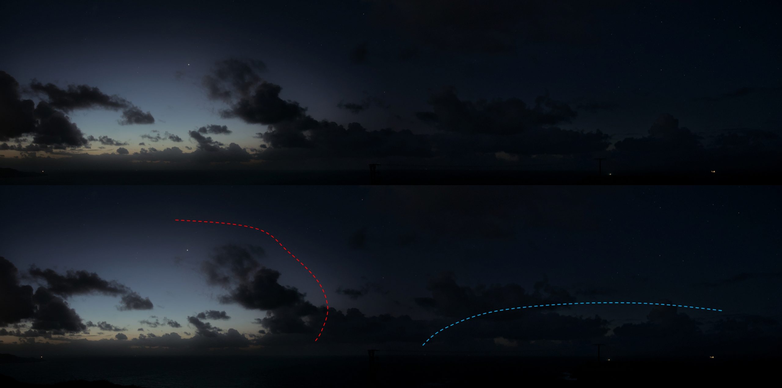
As the greatest eclipse approaches, the observer can see how the asymmetry in the sky’s surface brightness distribution gradually turns into a separated dark column, which starts to appear at the northwestern horizon, dividing the twilight glow into two distinct sections. The most peripheral section of the sky visible between the blue and grey lines is brownish, as it’s affected by the extinction. However, as the time was passing, it got brighter.

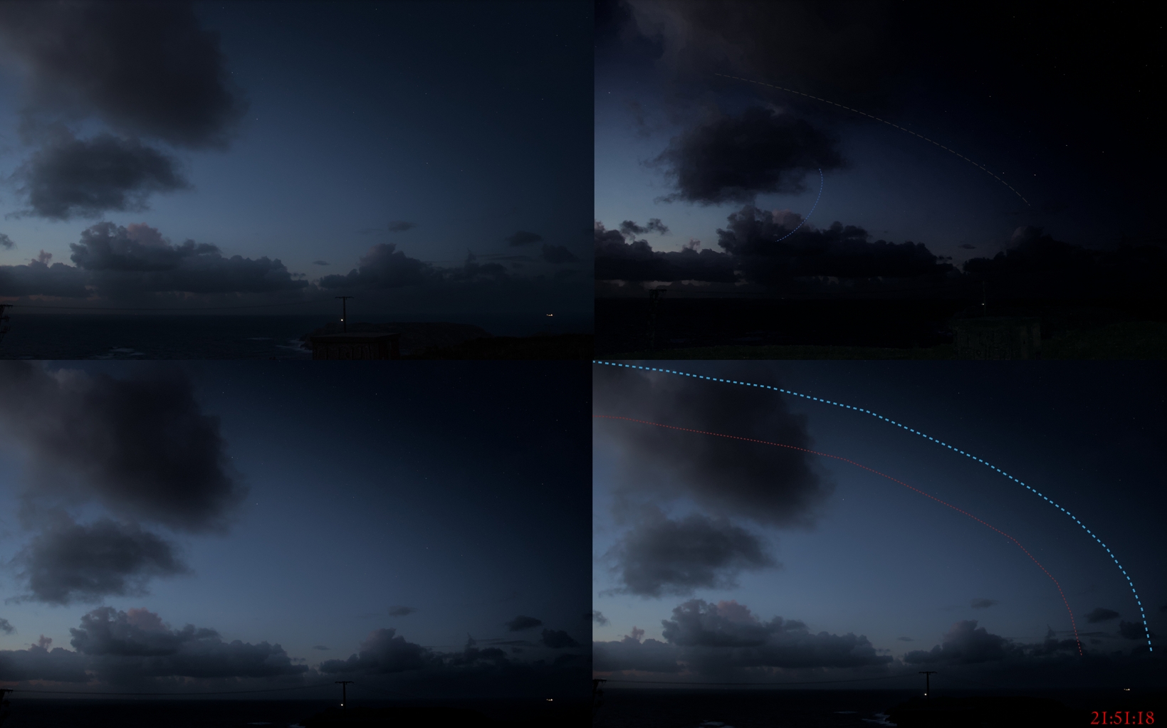
The effect is best visible in the top right image above (Pic. 55) where the contrast enhancement was maximized. A long line marks the boundary between the primary and secondary twilight, at which the sky surface brightness changes abruptly along with reddish appearance (red dotted line) discussed in the previous chapter. The most interesting is a somewhat perpendicular line, which marks the onset of the umbra. This particular matter is discussed in a further chapter. Notably, the western azimuth was a significantly brighter section of the sky, due to the smaller eclipse magnitude. The picture below shows abrupt changes in its right part driven by the proximity of the umbra (Pic. 56).

Except for the non-uniform distribution of sky surface brightness, there is a significant difference in overall sky illumination between these two images. It results in deeper threshold of stellar visibility, which corresponds to the deepest stage of nautical twilight at that direction and at least mid-astronomical twilight within the section of the sky, where the umbra was located (Pic. 57). Since the standard limit of visibility is about +1 Mag for typical twilight at this stage (solar depression of 8,6°) within the umbra this limit could be about +5 Mag.

The character of the changes is different when the eclipse magnitude decreases after culmination. The specificity of the impact on twilight differs because the increasing solar depression reduces the amount of scattered light being boosted by the shrinkage of the solar eclipse magnitude. An additional factor that shapes the spherical distribution of sky surface brightness is the movement of the area of greatest eclipse across the sky. This is an effect of the issue discussed in this article and briefly mentioned above. The area of greatest eclipse was moving southwards along the terminator line. It’s pretty well displayed in the animation of this eclipse available at Time and Date.com service and the next chapter. Alternatively, we can understand it by examining the graphs below (Pic 58, 59).

The situation like this reflects changes in the eclipse’s impact on the twilight glow, regardless of the solar depression. After the greatest eclipse, which was observable north of the solar azimuth itself, there is a moment, a bit later, when the same greatest eclipse occurs right above the observation venue, even though from an optical point of view, the whole appearance of the event is gone. At the direction of the sky, where the umbra was observed shortly before, the eclipse magnitude is a bit smaller than at solar azimuth. In light of this situation, we have the model A, considered earlier as one of a few, which characterizes the spherical distribution of sky surface brightness. By the way, worth analyzing are the values on the chart about the moment around T20:56:27 (Pic. 47), where the curved line briefly resembles the typical pace of sky darkening. This rough moment occurs roughly around the most significant eclipse phase observed at the solar azimuth, which is displayed later by another sky surface simulation adequate for this specific moment (Pic. 62). Directly before this point, an observer could see how the umbra fades out and “escapes” beyond the Earth’s atmosphere leaving analog sky surface brightness disturbance as known from example above (Pic. 54) but with much brighter northern section of the sky (Pic. 60-61).

The greatest impact of a solar eclipse on twilight can be expressed twofold, through the greatest eclipse visible from the location, expressed by the appearance of the umbra and all the optical phenomena visible along with it, and by the greatest eclipse at the location, passing the celestial zenith or solar azimuth. If the observer were located at the Bay of Biscay instead of Galicia, these two elements would be merged into one. In any other case, when the observer is outside of the extension of the totality, these two moments go separately. Depending on the location against the umbral path extension, one moment can be observed earlier than the other one. In my case, I could see the greatest eclipse visible at the location, as shown in the sky surface brightness distribution displayed above (Pic. 39) and the greatest eclipse at the location displayed just above (Pic. 62) in the bottom left image. The greatest eclipse visible from the location is treated as the counterpart of mid-totality, whereas the umbra was geometrically visible for 2m11s at the terminator line. Hence, the first sequence (top left image above) represents the moment about 50 seconds after the umbra left the Earth’s atmosphere and about 2 minutes after the aforementioned mid-totality. The moment at which the greatest eclipse, in fact, deep partial only roughly at my location, occurred 2 minutes later (bottom left image), and most of the isophotes are flattened. Two factors cause their asymmetry:
– decreasing eclipse magnitude towards the north direction,
– slight movement of solar azimuth northward since the eclipse began, as the field of view has a fixed direction.
The last rendering, about 5-6 minutes after the extended totality came to an end, stresses the asymmetry towards the south, where the eclipse magnitude was larger compared to the northern direction. In that particular moment, the impact of the greatest eclipse on twilight would be observed, i.e., in central Portugal.
Unfortunately, the proofs of both sky surface brightness and overall brightness after the greatest eclipse aren’t reliable enough because of increased cloudiness. The blocks of clouds visible far above the horizon finally came closer, but luckily, after the main eclipse spectacle (Pic. 63 – 66).

To summarize this section, we can examine the compilation of sky & scene brightness differences obtained from two separate observations, as per the guidelines proposed in this article (Pic. 67).

Reports are scarce after the eclipse’s culmination between 22:12 and 22:31. Although images were taken, the significant cloudiness prevented them from being of sufficient quality to be presented in this comparison.

6. UMBRA MOVEMENT IN THE SKY

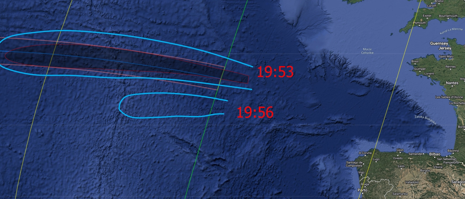
The presence of the umbra is undeniably the key moment of the solar eclipse observed below the horizon. It marks an enormously larger impact on the twilight sky than the surrounding, even adjacent areas, which catch even the smallest piece of direct sunlight. This is because the twilight sky is at least once shadowed and even double shadowed as far as the secondary twilight is considered. However, the crucial altitude considered is 40 km, and we should expect the greatest effect only within the primary twilight zone, which doesn’t change the fact that the same altitude located directly beyond the terminator zone will also be affected. As the section of the sky is completely shadowed, it receives only the sunlight scattered by the adjacent sections of the sky. Before I get to this point, there is one noteworthy thing. The umbra behaviour at the terminator is entirely different from that observed around the point of greatest eclipse. This particular matter will be elaborated in the future, although for now let’s understand it in the following way, where the greatest eclipse point umbra is the closest to the circular shape, next as it gets closer to the terminator line, it becomes more oval with increasing tilt of its central axis. Since the major axis of the umbra near the greatest point of the eclipse has the meridian placement, the same major axis of the umbra at the terminator line has the parallel placement. The primary consequence of it is the way the umbra moves across the Earth’s surface. The first one moves along the eclipse path, although as it approaches the terminator line, it breaks this rule and moves against the eclipse path, perpendicularly to the line marking the greatest eclipse. The animation on the left shows how it looked on April 8, 2024, in the North Atlantic Ocean (Pic. 68), and a similar situation was illustrated in this article.

The Moon’s shadow, which by definition should proceed from the west to the east, at the end of its path moves somewhat southwards. There are two reasons explaining it. Firstly, as one of the umbral “vertice”, which ends up the central axis goes into space, the umbra becomes thicker. Secondly, as the major axis is seriously tilted, it eventually imitates the perpendicular movement of the shadow. Noteworthy is also the last moment of umbra appearance, when its last “vertice” leaves the Earth’s surface, because its position indicates the tail end of the major axis, which lies in an opposite place against the line of greatest eclipse. The direction of umbral movement roughly at the terminator line depends on at least two factors:
-> Position of the greatest eclipse point against the sub-solar point – when the eclipse point is located north of the sub-solar point, then the northern end of the main axis shifts from NW to NE directions as shown in the graph below (Pic. 61).

The explanation of it can be found in analyzing the speed of the umbra on the Earth’s surface. As it comes to the terminator, its speed is the highest. The same applies to both sides of the umbra. If the given side of the umbra is closer to the sub-solar point (B), it moves more slowly than the opposite side of the umbra (A), which, by definition, will move a bit quicker. In turn, the orientation of the umbra over the whole eclipse path will change. Eventually, at the very end, we might have an impression that the umbra moves perpendicularly to the eclipse path, like the animation above shows us (Vid. 2). This is, anyway, the topic for further, more detailed explanation.
-> Nodal position of the Moon – plays a minor role here and might alternatively decide about the distance of umbra egress/ingress against the central line of the eclipse.
-> Placement of terminator line against the illuminated hemisphere – the apparent movement of umbra at the terminator line will have opposite directions against sunrise and sunset.

The umbra ingress at the terminator line is more complicated from an optical point of view. One of the reasons is explained directly after this article. The second reason lies in the specificity of the solar eclipse, which behaves analogously to a logarithmic function. It means that the areas directly before the second contact are significantly darker than others, despite the fact that the umbra itself isn’t visible yet. Good example is shown in the image below (Pic. 62). which determines the darker area in the sky affected by the deep partial phase of the eclipse just before the umbra approaches.

The animations below show how the umbra meets the terminator line as the total solar eclipse ends up on the Earth’s surface.

Due to cloud interruption, the observer was unable to see the entire umbral behavior, which is why the Stellarium 25.2 ShowMySky animation for the same location has been applied below.

Finally, the animation aboveshows the apparent movement of the umbra somewhat alongside the terminator line, which states the boundary between the primary and secondary twilight sky. The umbra optically moves perpendicularly to the path of totality as discussed earlier. An observer could see it less expressed because of clouds, although the twilight glow visible on the left is apparently shrinking in account of the moving umbra.
At the end of this section, there are some panoramic images, which show the umbra position around the mid-totality observed at the northwestern sky (Pic. 64 – 66).

As well as the umbra position according to the Stellarium 25.2 ShowMySky mode (Pic. 67) for Malpica, where the observation took place, and the Carino, close to which the observation was planned initially.

In summary, the entire sequence of umbra movement is presented in the images below. They’re modified in various contrast enhancement (Pic. 67).

The whole sequence shows the movement of the umbra as well as the rapid changes of the adjacent section of the sky affected by the deepest eclipse phase, resulting in various coloration bands, which are a subject of discussion in the next chapter. Moreover, we can see the approximate position of the twilight wedge with a dark secondary twilight sky beyond.

7. UMBRA LIMIT COLORATION

The visibility of the umbra within the primary twilight section of sky is not confined only to the significant difference in local sky surface brightness. Its apparent view seems to be more complicated, as the observer can see the asymmetry in the coloration of the umbra limit. The problem was observed already in 2019 during the first webcam observation of a total solar eclipse below the horizon. Moreover, it was explained pretty much well as far as this one example was concerned. The image below illustrates what the phenomenon looked like in Malpica last year (Pic. 69).

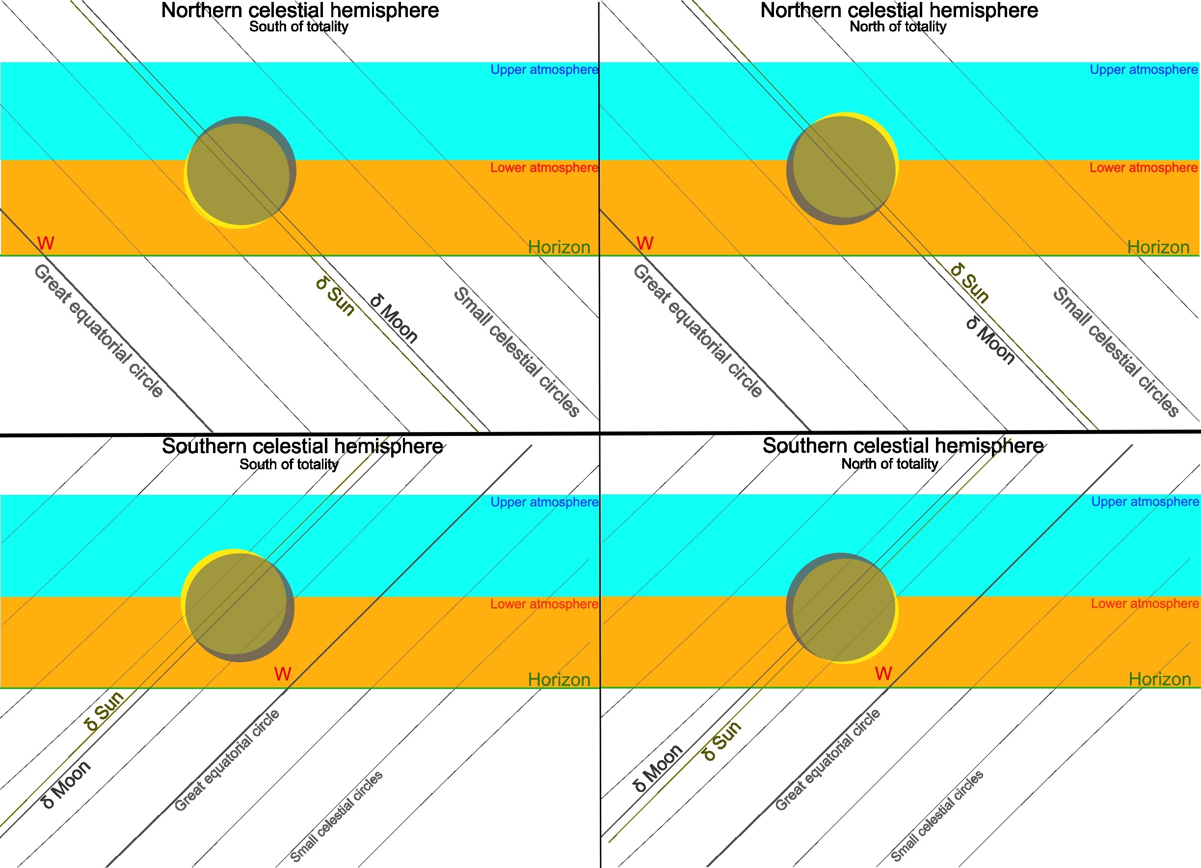
Admittedly, the configuration of the color bands is the same as observed in 2019, although an observer in this case is looking at it from an opposite direction. Since the July 2, 2019 observation was made at solar depression of circa 1 degree towards antisolar direction, the April 8, 2024 observation was conducted at solar depression of 8,6° towards solar azimuth, in both cases, the observation venue was placed offside to the umbra extension, which definitely means different perspectives of both umbra limits observation. The phenomenon requires deeper analysis, which should include the nodal position of the Moon, the character of lunar shadow ingress/egress, and eventually, the latitude of the observation. Since the first two will define the estimated position of the 2^nd and 3^rd contact against the horizon, the last one will determine the position of the equatorial system against the local horizon. There are two types of coordinate systems used in spherical astronomy: equatorial and horizontal. Equatorial determines the angular distance of an object from the celestial equator, which is called declination. The angular distance from the vernal equinox, eastwards along the celestial equator, is called the right ascension, which isn’t essential here, likewise the azimuth in the horizontal system. A crucial value in a horizontal system is the altitude. The graphical representation of the difference is shown below (Pic. 70). 

Now, it’s easy to visualize what happens at the equator. The “horizontal grid” is perpendicular to the “equatorial grid”. Conversely, both systems are aligned perfectly with each other at the poles. Since the eclipse happens at some latitude between the equator and the pole, the celestial equator with the entire system is tilted by the angle, which represents the difference between the zenith and the value of latitude. Since the latitude of the equator is roughly 0°, the celestial equator will be oriented 90° against the local horizon. Because this eclipse effect was observed at a latitude of 46-47°, the celestial equator is tilted by 90-46 = 44 degrees with the local horizon. At other declinations, the following angle can be computed in the same way as the path of the stars.  The way in which the great circle and small circles cross the horizon is illustrated below (Pic. 71).

 

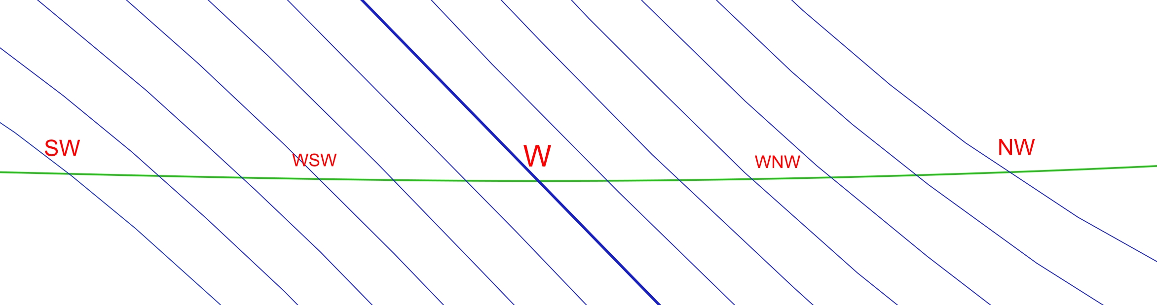
Imagine that every single line illustrated above (Pic. 71) represents the path of an exemplary star. You can recall various startrail images. Each single trail represents the celestial movement of an object at a certain declination. The same is here. The thickest line marks the celestial equator with declination equal to 0, whereas other lines are simply paths of objects with declinations other than 0. Translating it into the eclipse situation, we have two celestial bodies contributing to the event: the Sun and the Moon. Both have separate declinations, unless we consider the brief moment of mid-totality with an umbral depth of 100%. In the vast majority of cases, the Moon has a slightly different declination than the Sun, which is the key to understanding this optical phenomenon. The declination of the Moon during the eclipse keeps changing as per its nodal position. For the descending-node eclipses, the Moon’s declination decreases, whereas for the ascending-node eclipses, the Moon’s declination increases. These changes are relatively minor in the span of just a few minutes of totality, so that we can treat them as a supplement. Returning to the second reason, which determines the ingress and egress of the shadow, the pivot role is being played by the size of umbra and its position against the subsolar point (Pic. 61). Finally, the difference in declination between the Moon and the Sun will contribute to the position of contacts as well as the crescent sun orientation outside of total phase. As this text might be too complicated, refer to the graphic interpretations below (Pic. 72 – 74).

The difference in declination between the Sun and the Moon results in the crescent position at the eclipse culmination against the horizon and thereby the thickest section of the Earth’s atmosphere. As noted earlier, the atmosphere at an altitude of about 40km looks optically “compressed” (Pic. 33). The solar disk is far larger than the apparent layer of the atmosphere at this altitude. When the crescent is oriented with both horns away from the horizon, the limb darkening effect is enriched by the behaviour of Rayleigh scattering in a thick atmosphere, which by definition results in scattering of long wavelengths. Conversely, for the crescent sun with both horns turned into the local horizon will feature a somewhat subdued limb darkening effect, as the light passes a significantly thinner atmosphere with a weak influence of Rayleigh scattering with short wavelengths only. The dependence of the Sun’s crescent position on certain latitudes and nodal positions is another noteworthy thing. By default, the crescent Sun orientation is pretty much perpendicular to the small celestial circles. In light of it, the latitude determines the direction of the crescent. However, it’s not the only thing, as the nodal position of the Moon also plays an essential role. In fact, the images above (Pic. 72) aren’t meticulous enough to show it. Still, depending on what type of node the eclipse is observed, the additional shift of the crescent can be observed east or west of the hypothetical perpendicular line, which is stated as its symmetry axis. A good example is the Devil’s horns observed on the last deep partial solar eclipse in Canada. That eclipse was on the ascending node so that the crescent position could produce the effect. Usually, it would look slightly diagonal. Anyhow, it’s just a digression by now, which leads to the conclusion that the latitudes probably enhance the initial discrepancy of umbra limit coloration. The entire event isn’t confined only to the greatest eclipse phase. It occurs dynamically along with various positions of contacts. As the umbral depth increases, the position of II^nd or III^rd contact is observed closely to the angular diameter of the Moon’s disk. The same as in the case of a deep partial eclipse, these contacts are location-dependent, as shown in the images below (Pic. 73).

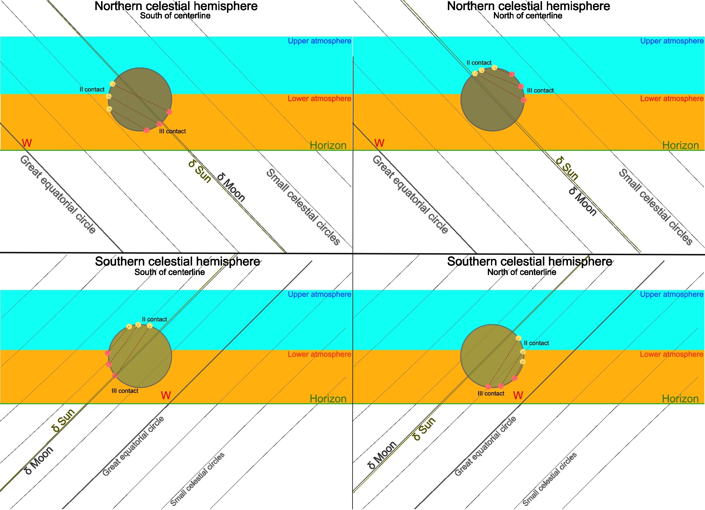
Everyone located south of the centerline should see an enhanced reddish band caused by both contacts. In contrast, observers located on the opposite side of the centerline will see the reddening at a later stage of the eclipse. For them, initially, the umbral limit will feature a bluish band with a slight shift towards red, as the umbra proceeds towards the south. The common denominator will be a thin solar crescent with both horns up located at the horizon line, through which light will be passing the thickest section of the atmosphere, resulting in intense reddish coloration. This phenomenon proceeds immediately after the umbra leaves the Earth’s atmosphere (Pic. 34). Since the eclipse happens at sunrise, everything will be in reverse sequence. The intense reddening will precede the umbra ingress directly into the atmosphere. Finally, let’s see what happens roughly at the centerline. The position of the contacts isn’t apparent. They don’t follow the small celestial circles, as the nodal position of the Moon also defines them (Pic. 74). Assuming the same eclipse circumstances for different nodal positions, the difference in umbra limit coloration seems to be more expressed at the ascending node eclipse, at least as far as the sunset is considered. The sunrise wasn’t analyzed this time, as the work revolves between the 2024 and 2026 solar eclipses visible from Europe around sunset.

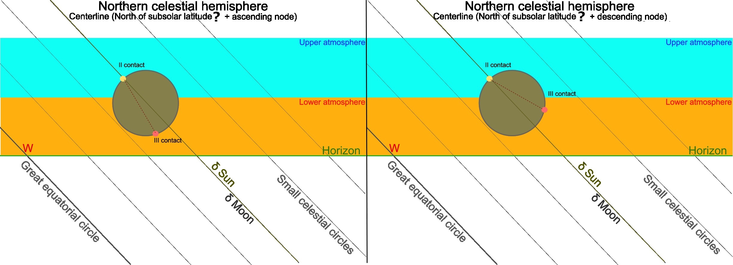
Translating it into practice, worth attention is the image below, which compares the eclipse view for two positions located on both sides of the path extension. Imagine that you are floating 35-40km above the ground, and what exact eclipse phase you can see from there (Pic. 75).

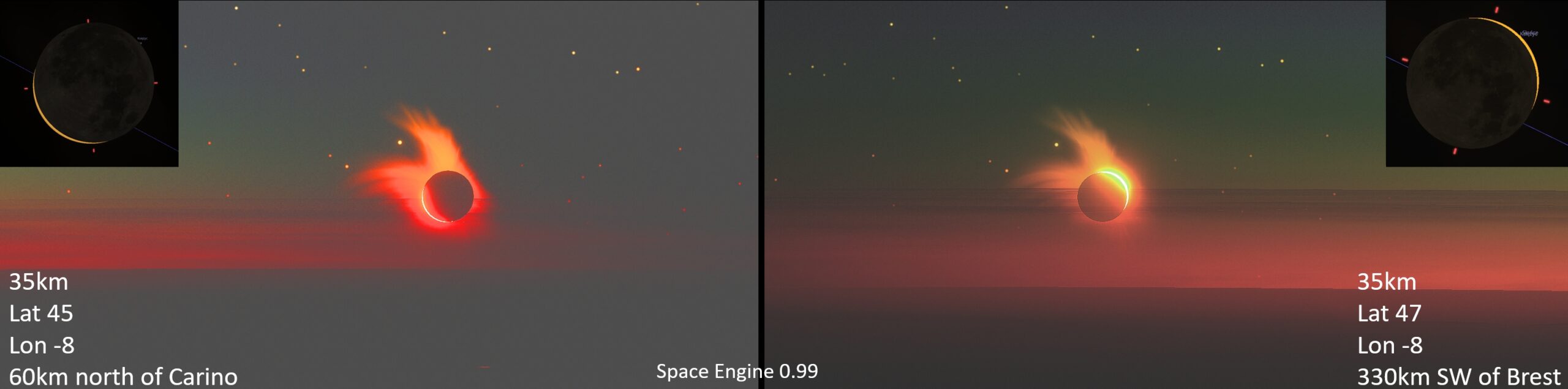
An observer from this altitude could see the crescent Sun shining within the thickest section of the atmosphere just above the horizon or slightly above, in the opposite case, when the slim crescent shines through a thinnier atmosphere. These opposite circumstances shape different conditions of Rayleigh scattering, which contribute to the final color bands observed at the edges of the umbra. The illustrations above (Pic. 73, 74) apply to the situation, from which an observer could watch the eclipse from the same altitude, but within the zone of totality. Besides the things listed earlier, we can’t forget about the umbral depth, which will determine the positions of eclipse contacts locally (Pic. 73, 74). As a result, over the horizontal totality such as this, in some cases, the 2^nd contact will be observed on the lower part of the limb, within the thickest section of the atmosphere, leading to an enhanced limb darkening effect. Threading this way, the reddish band can be eventually observed on both sides of the umbra as the totality progresses (Pic. 76). The 3^rd contact always appears closer to the horizon, which has its geometrical explanation discussed on earlier occasions. In an outcome, the elusive umbra will always be followed by an extended reddish band zone reported earlier in this article (Pic. 34).

 

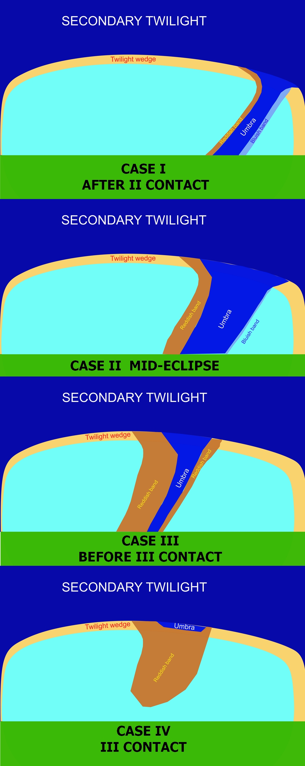
As the eclipse progresses, the color discrepancy is fading out. Eventually, an observer can see the reddish tinge on both sides of the umbra. The very last moment shows the intense red shift in the place where the umbra was observed seconds earlier. Next, this zone moves southward and weakens. As discussed in previous article and the chapter above, this is related to the penumbra oval and changes of the eclipse gamma value. Unfortunately, all the theories presented in this whole chapter do not seem to be enough for the explanation of this phenomenon. According to the Stellarium 25.1 ShowMySky model, the umbra limit color disparity increases as we move away from the extended eclipse zone in all directions. As per the model, it’s not observed only when the observer is placed precisely within the totality extension, when the solar azimuth, which scatters most of the light, is shaded. If this is so, the reason for this coloration could be related to the coloration of the antitwilight sky, especially since they look very similar to the Belt of Venus. This problem will be undertaken on the 2026 total solar eclipse with the hope that the final explanation will be applied.

 

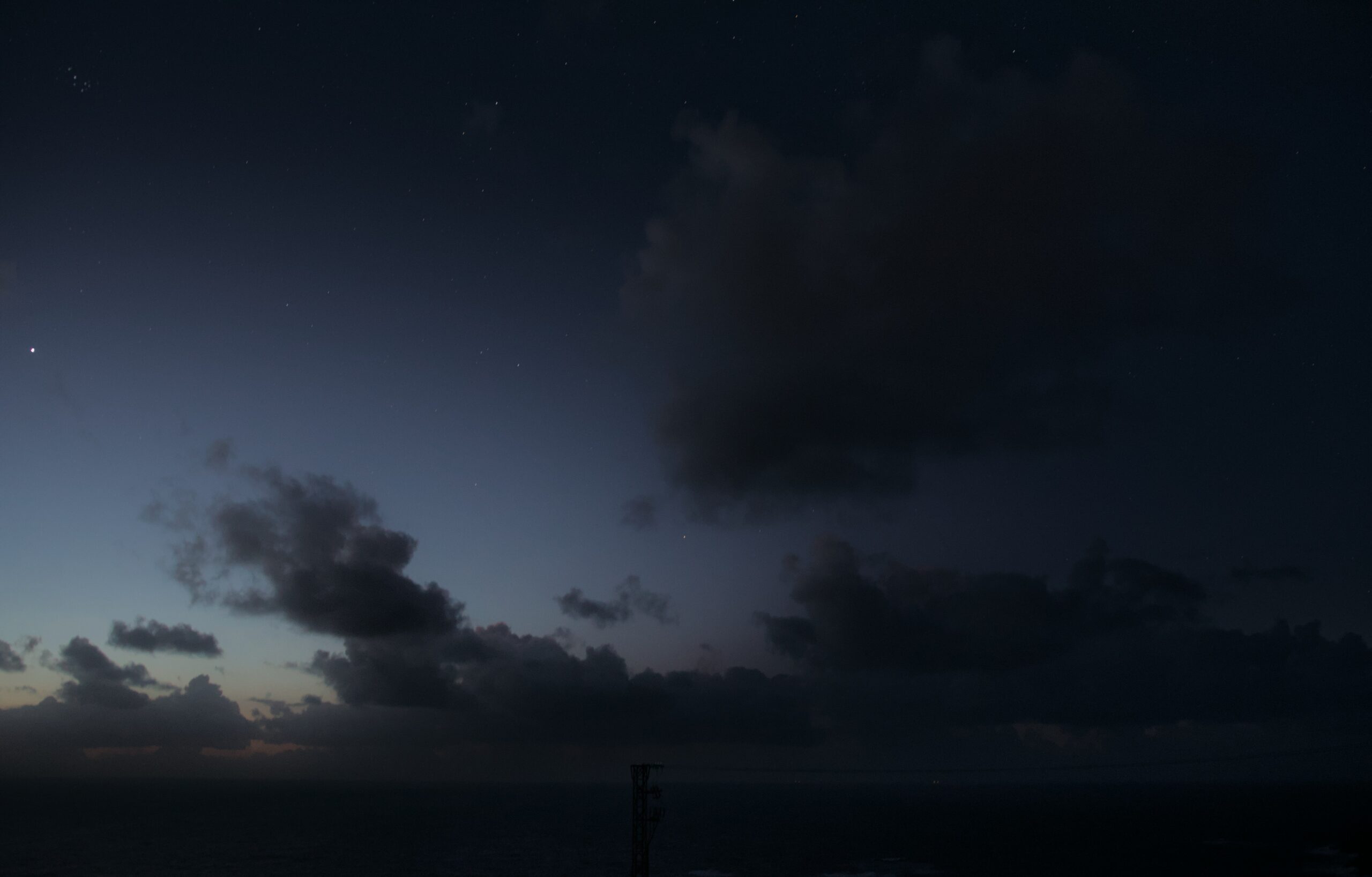
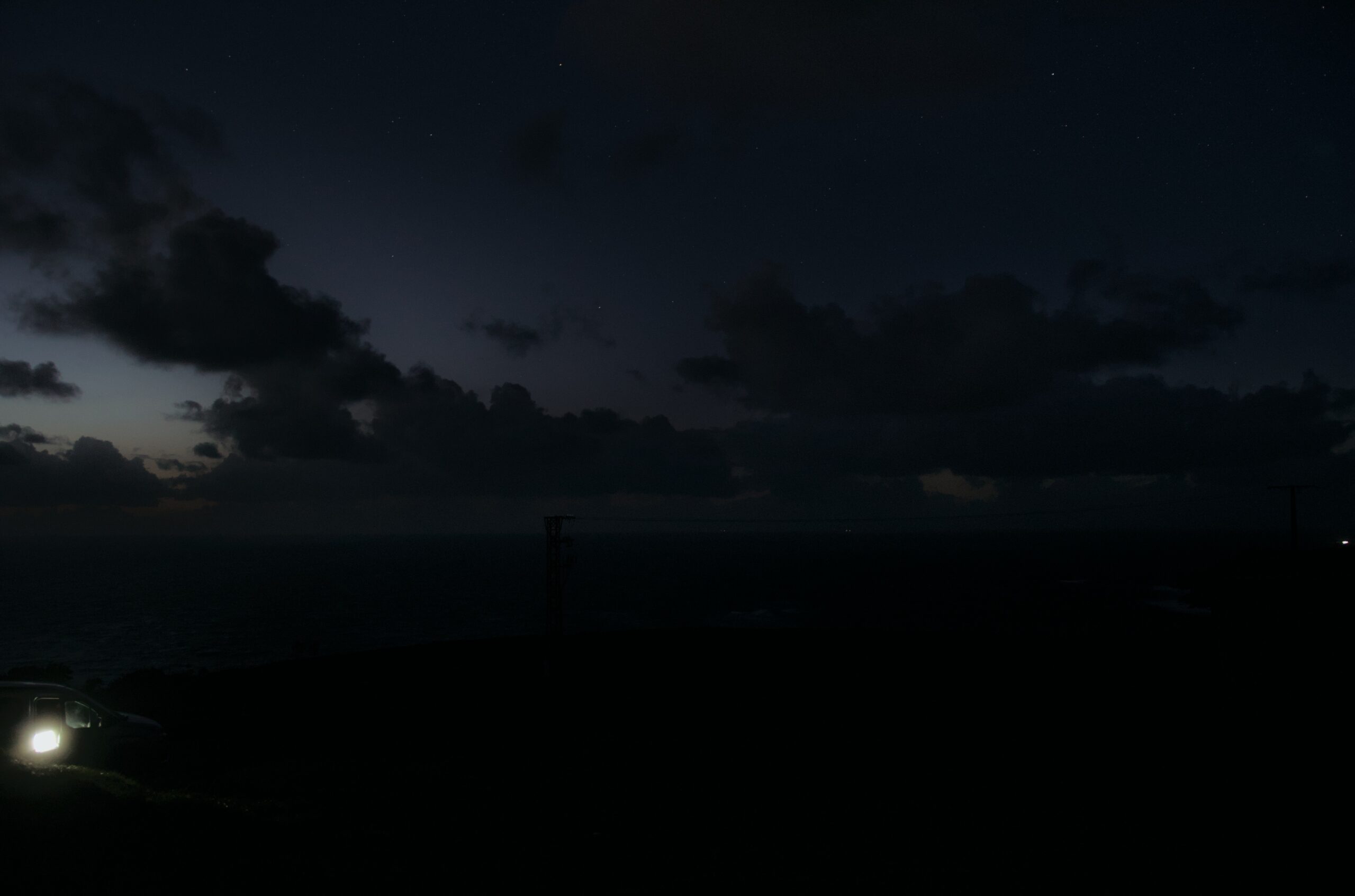
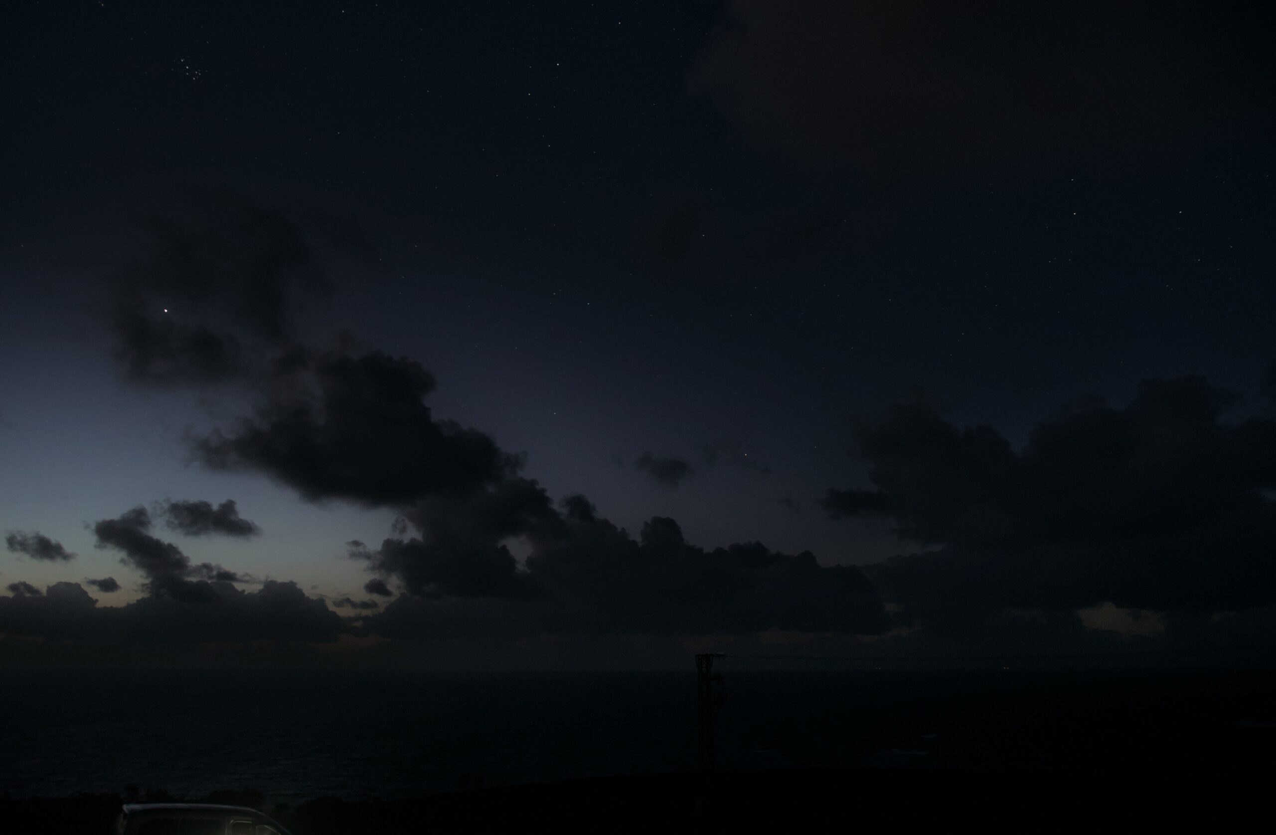
8. SECONDARY TWILIGHT

The zone of secondary twilight represents the sky already engulfed in the Earth’s shadow, placed beyond the twilight wedge, which marks rapidly weakening direct solar rays in illuminating the lower atmosphere. Unlike the primary twilight zone, being directly penetrated by the rays of the setting Sun, which serves as the sole source of illumination, the shadowed section of the sky is illuminated at most by the light scattered in the sunlit part of the Earth’s atmosphere. The secondary twilight sky, being submerged in the shadow, no longer contributes to the sky brightness. The scattered light comes at most from the higher part of the atmosphere, which still catches the rays of the setting Sun, but because the air density drops rapidly with height, the scattering coefficient also drops, sunlight is scattered increasingly more weakly, and the sky brightness diminishes (Rozenberg, 1966). The second-order scattering begins to become important at the boundary between the civil and nautical twilight, which in our case corresponds to the influence of a partial solar eclipse with the magnitude exceeding 0.7. As the shadowed region of the sky is illuminated by the radiation from the sky, particularly from the azimuth towards the Sun, theoretically, the influence of a deep partial eclipse such as this should be noticeable. Hypothetically, as discussed on the occasion of the solar eclipse of December 14, 2020, below the horizon in Namibia, the most significant impact should apply to the section of the sky located directly beyond the umbra location. It would mean the lowest amount of second-order scattering exactly at solar azimuth in a hypothetical place 40 km above the ground, where the Sun is already below the horizon. Considering the solar depression of 8,6° at the greatest eclipse, the direct solar beams would reach only the upper atmosphere at the estimated altitude of the turbopause once the zenith sky is considered. However, there was still a large shadowed section of sky at the solar half of the twilight sky, where the umbra extension could theoretically be visible following earlier hypotheses. In fact, the density of the atmosphere decreases significantly with height, so even if the upper part is still directly illuminated by the Sun, the number of particles isn’t big enough to scatter this light down to the ground. At least it yields secondarily scattered sunlight in the lower parts of the atmosphere, intensively illuminated by the Sun being already below the horizon. Therefore, the presence of an umbra should optically diversify this amount of scattered light and make it visible to the observer. The observation made on April 8, 2024, verified them, as no changes within the secondary twilight have been proven. When solar depression exceeds 8°, the atmosphere lying within the shadow of Earth is illuminated secondarily by a still intense twilight glow. However, even if this glow is interrupted by the umbra, the light comes from adjacent parts of the sky, where the crescent Sun operates all the more so that the umbra is significantly brighter than the sky shadowed by the Earth. Assuming that the apparent magnitude of a total solar eclipse is about -16, we experience the conditions nearly 40x brighter than the full Moon. Consequently, the presence of umbra probably doesn’t continue within the sky, which isn’t directly illuminated by the Sun. It doesn’t change the fact that further similar observations are desirable, especially within the astronomical twilight zone affected by the eclipse. According to Stellarium 25.1 ShowMySky mode, the apparent visibility of the umbra is detectable at solar depression of nearly 15°, which basically corresponds to the limit of “true dusk”.

 

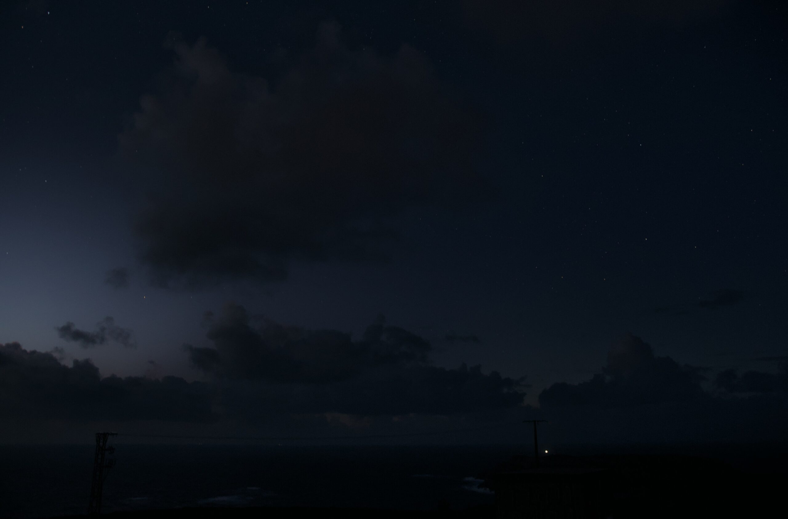
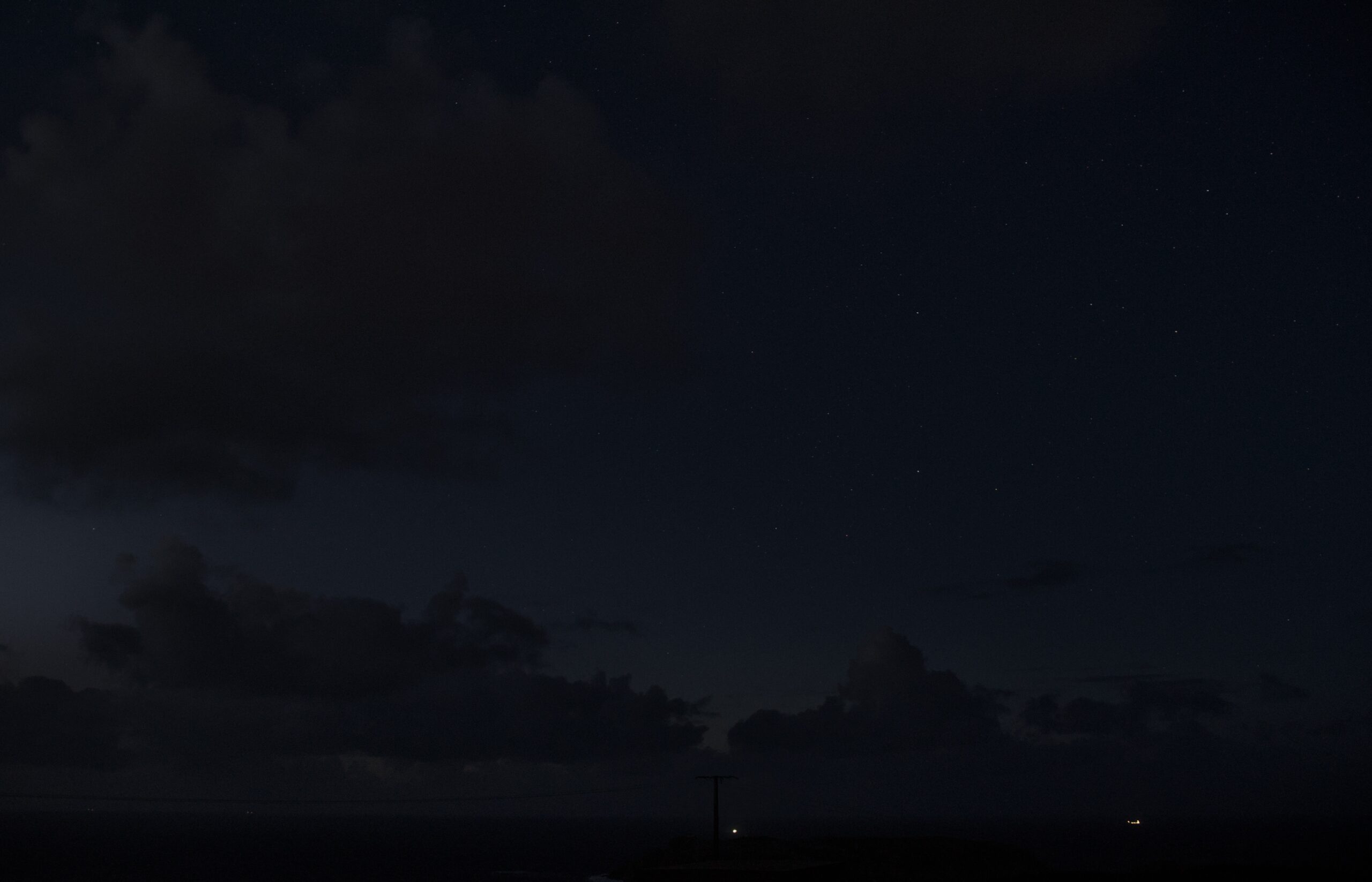
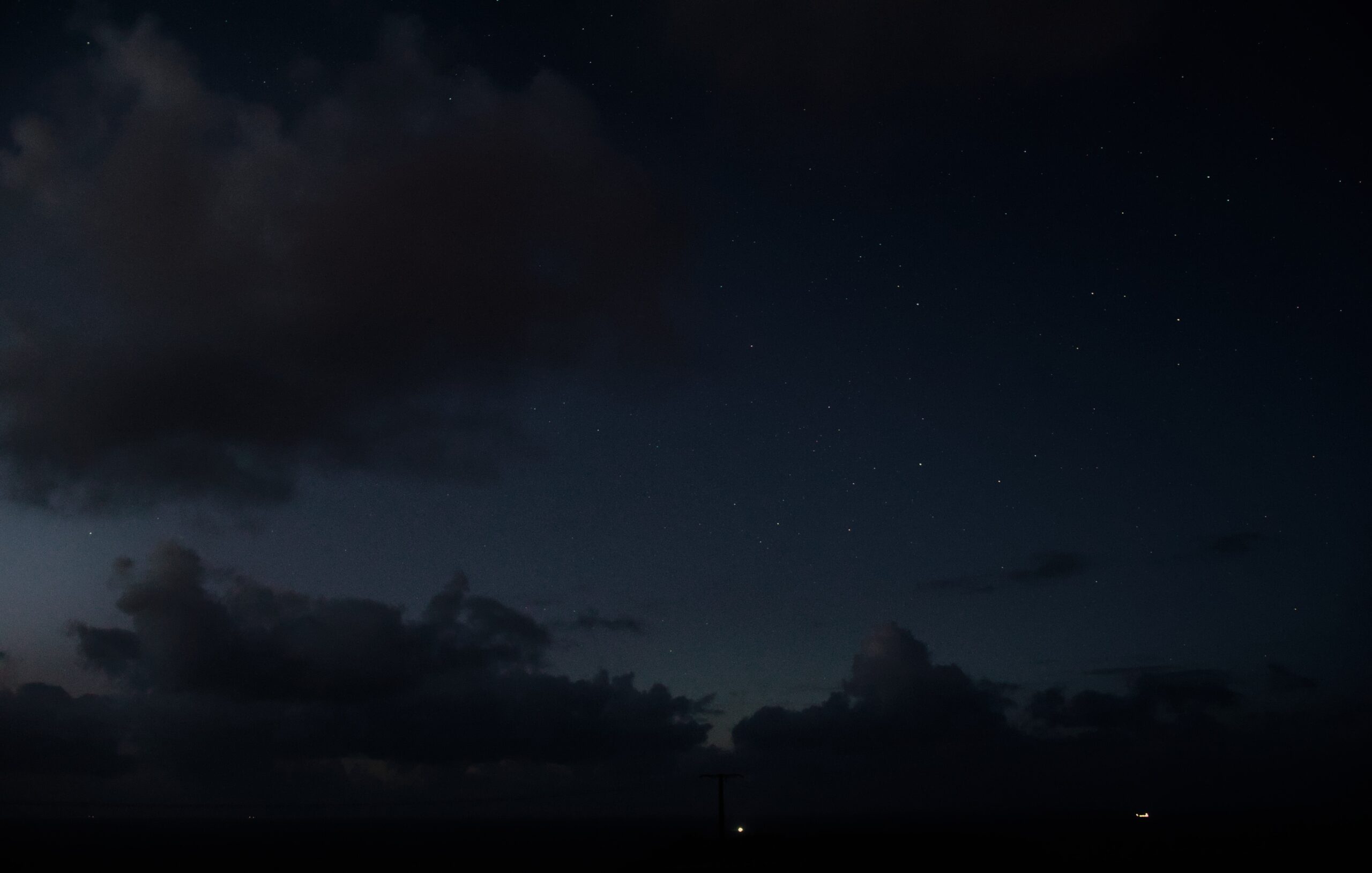
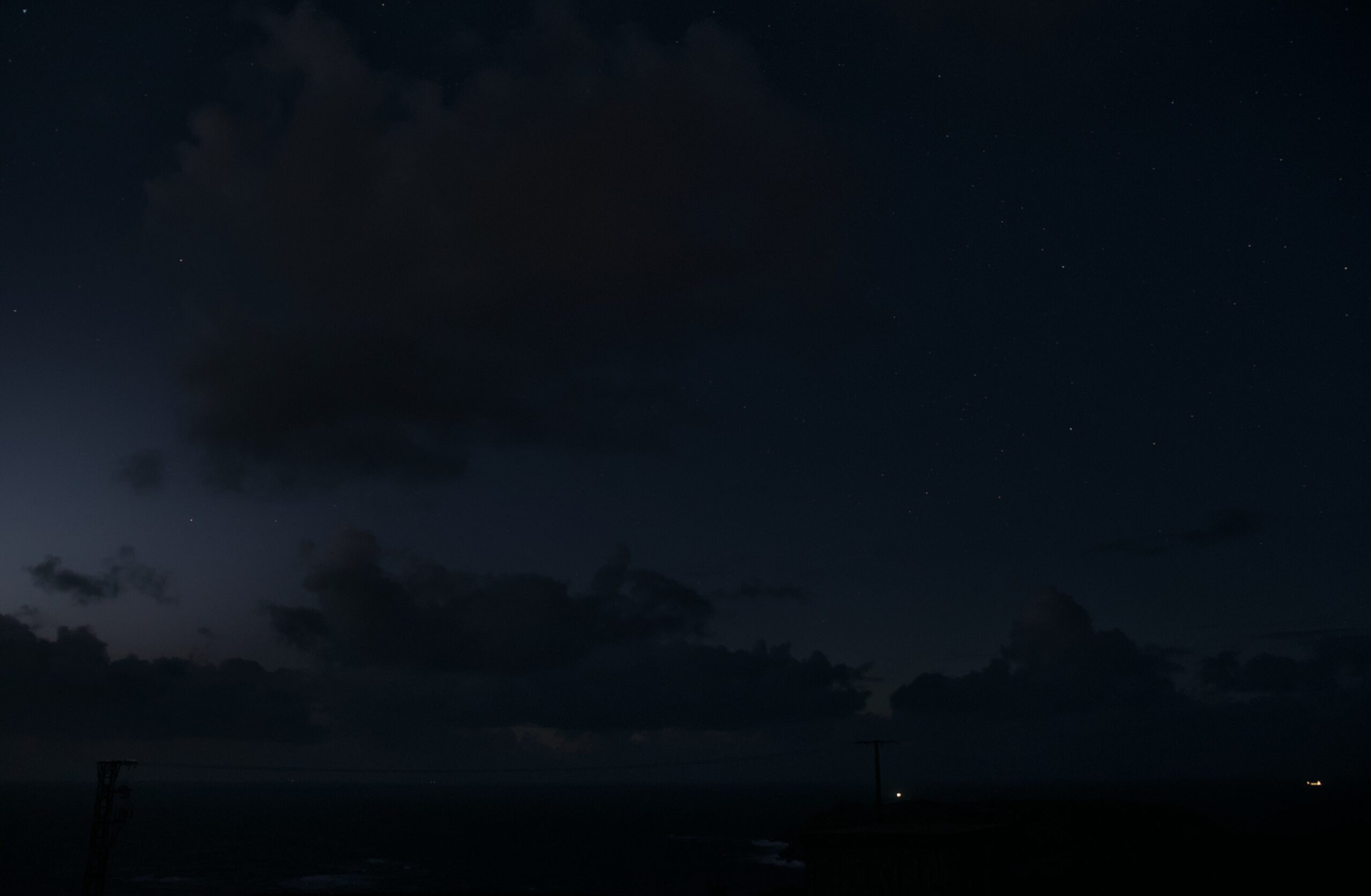
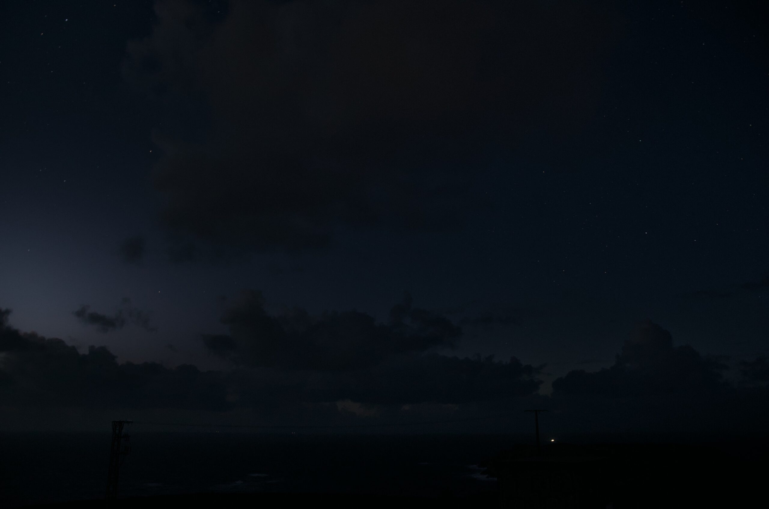
9. OTHER ASPECTS

There are additional threads to be explained next to the aspects described so far. At first, the crucial element is the varying times of eclipse culmination at different locations along the terminator line. The problem has already been illustrated above (Figures 58, 59) in the context of explaining the umbra behavior. Following the various speeds of umbra, illustrated, i.e., by its tilted axis (Pic. 61), we should imagine the same for the penumbra in any size restricted by the curves of the same eclipse magnitude. Let’s have a look at the same image from a broader perspective, which covers the isolines of the greatest eclipse moments in the UTC (Pic. 87).

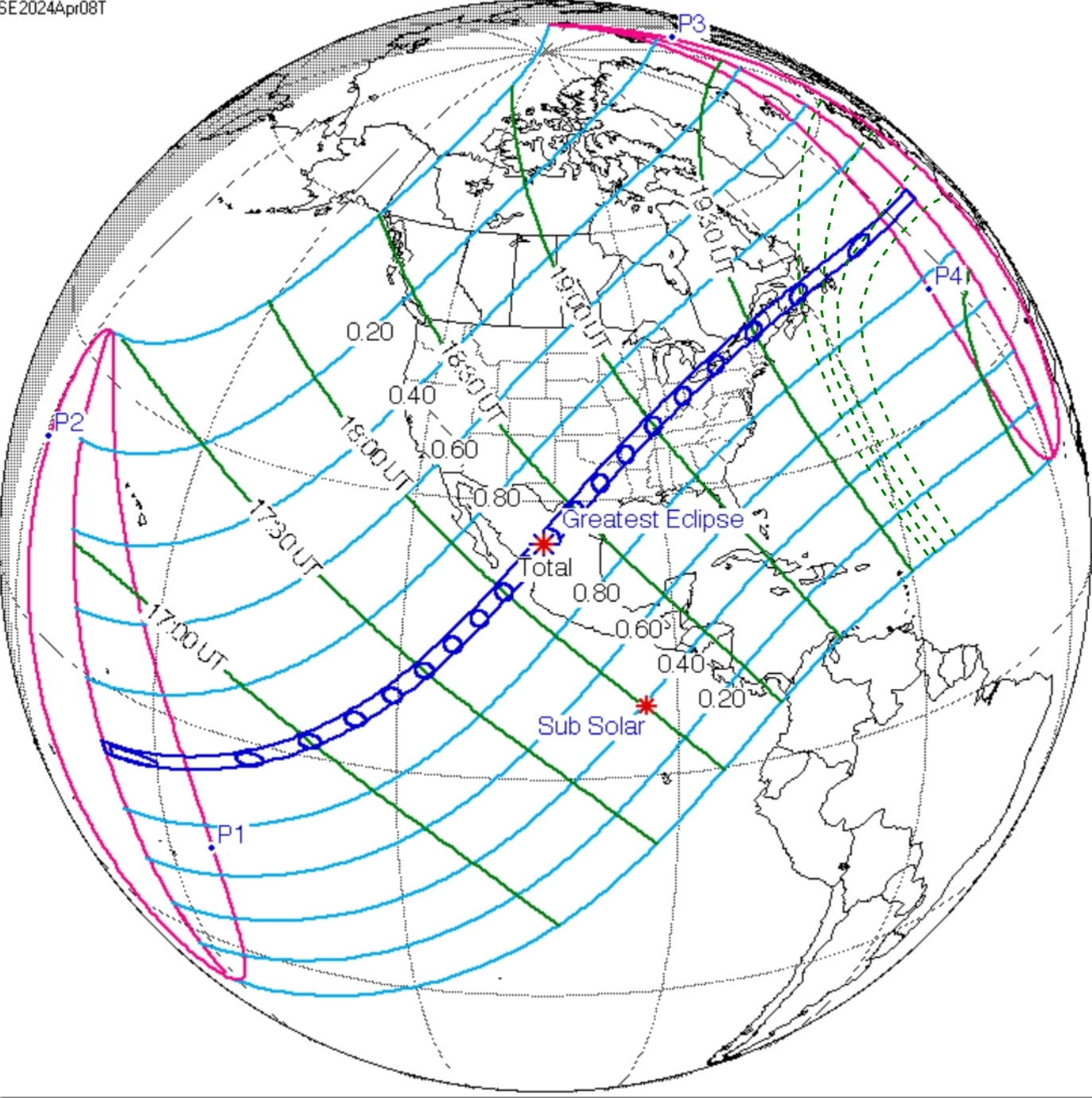
For a better imagination of this phenomenon, we can watch the animation below (Pic. 88).

The moment of greatest eclipse moves southward at the sunset’s terminator line. An opposite direction would be observed at sunrise. It practically means that the moment of greatest eclipse, expressed mainly by the presence of the umbra, wasn’t the moment of the greatest eclipse for some locations at which the umbra could be observed! By looking at the sequence of images below, we can clearly understand what it looked like in Spain last year. Before the umbra became visible, the northernmost section of the primary twilight sky was considerably darker and then got brighter as the eclipse progressed. Additionally, the movement of the umbra from north to south (Fig. 63 and videos below) was a consequence of this visualized event, indicating the direction of the eclipse’s progress.

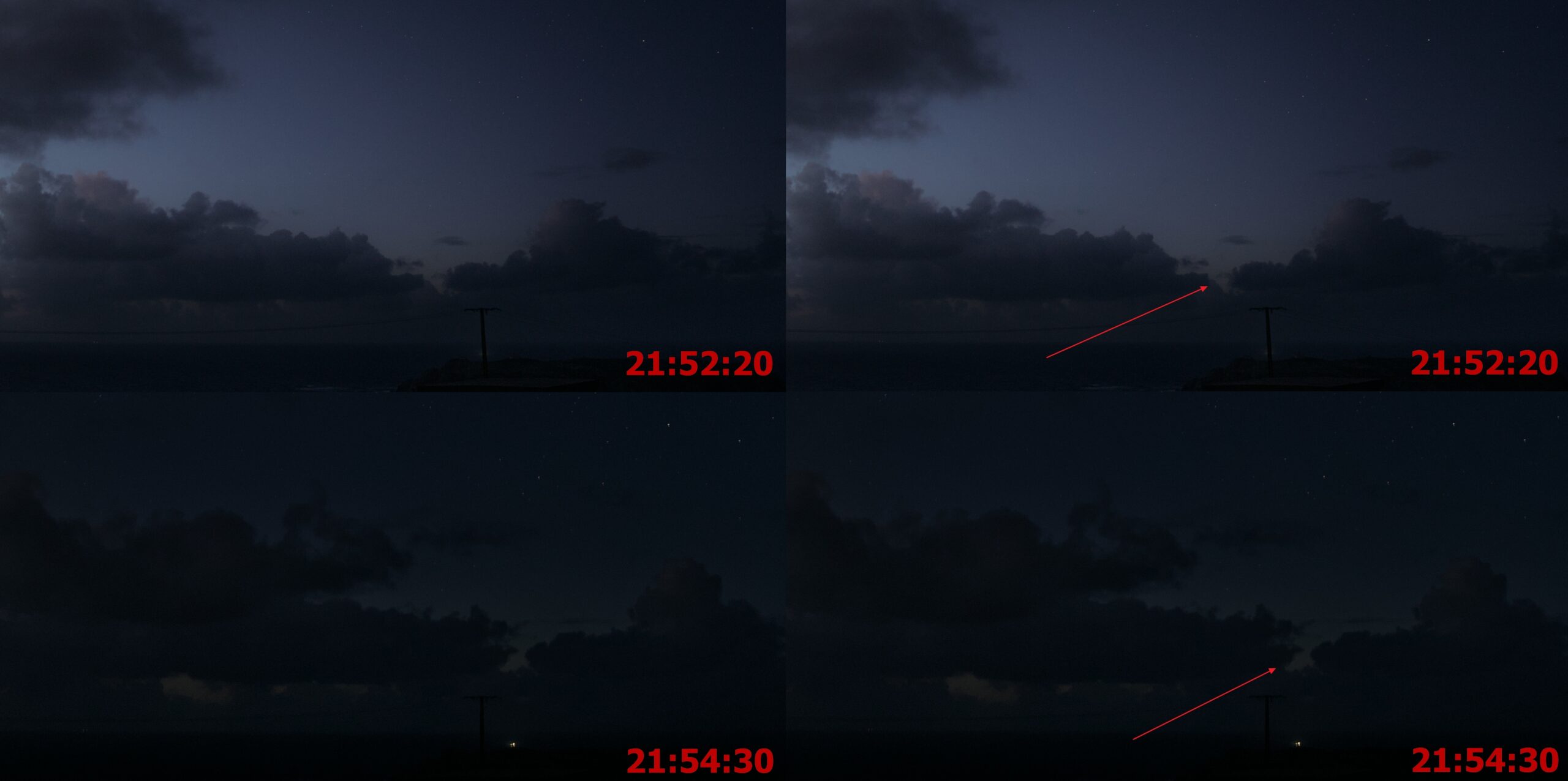
The most distant sky in the NNW direction was partially obscured by the moving clouds, which eventually created a useful contrast. Initially, shortly before the umbra started to appear, an observer could see a slight darkening of the sky in that direction. It was the moment of greatest eclipse north of the path extension, where the magnitude could reach about 0.98-0.99. Once the umbra became visible, this particular section of sky started to get brighter. Initially, it happened slowly, but later it became a rapid phenomenon. From an observer’s point of view, it was like something with the brightness between the Sun and Moon was about to rise in that direction shortly. When the eclipse culminated at the extension of the centerline, the eclipse magnitude in that section of the sky could be comparable to the estimated magnitude at the observation venue. It’s just an assumption without any computations, which is aimed at making all of you aware of the dynamics of the eclipse phenomenon at the terminator line. The specificity of isolines with the greatest eclipse impact on twilight will be explained in further readings. According to the map above (Fig. 58), at my location, the greatest eclipse occurred only about 30 seconds later than at the point where the centerline intersected the terminator line. However, it applies only to the zenith sky. Each section of sky experienced a different moment of eclipse culmination, which is illustrated in the image below (Pic. 90).

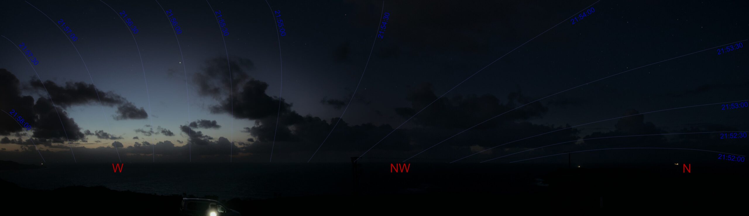
This situation also explains the moment of the most significant eclipse impact on the sky surface brightness in the direction of measurement. As presented above, the Unihedron device was oriented at nearly western azimuth, the biggest impact was reported more later than the observed eclipse culmination itself (Pic. 91).

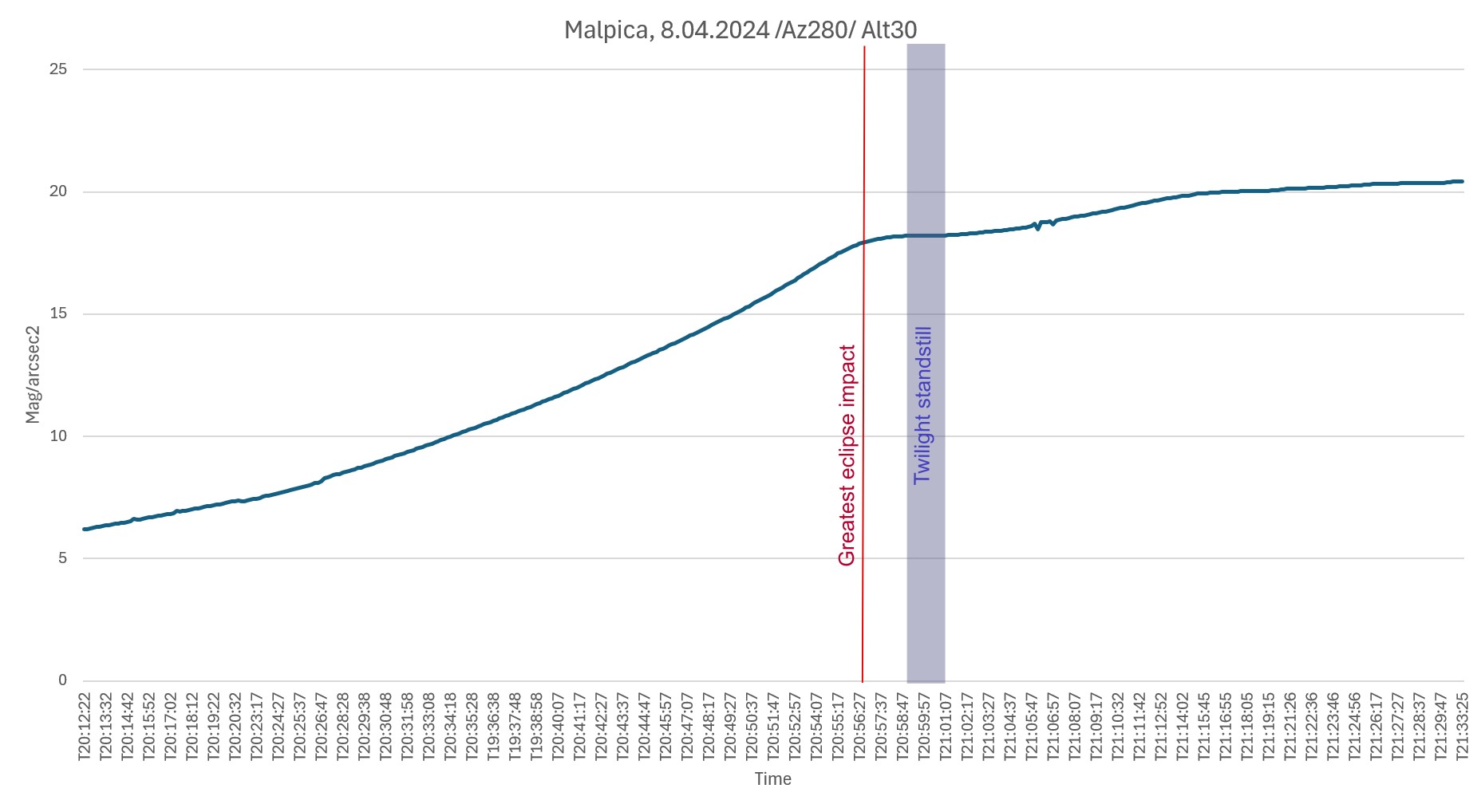
According to the Unihedron SQM-LU-DL device, the largest impact of the solar eclipse on twilight at an azimuth of 280° occurred around 20:56:30 local time, so over at least 1m30s after the umbra disappeared. Why did it happen like this? The answer is presented in the map below (Pic. 92) modified from above (Pic. 58). As the isolines with time indicate the moment of greatest eclipse impact, it doesn’t happen on the same time everywhere, thereby in each section of the sky at once. Since the northernmost sections of the sky already experienced the eclipse culmination, the sky sphere in the western direction is still “awaiting” it. The culmination eventually arrives and represents the magnitude suitable for local circumstances. When the impact of the total solar eclipse was visually observed in the northwestern direction, the azimuth at which the measurement was taken represented the impact of a deep partial solar eclipse with approaching culmination. It proves the other point, that the estimation of eclipse obscuration or magnitude below the horizon will never be accurate or uniform. This is because the direct sunlight scattering doesn’t take place, and the light level distribution over the sky is more complex. The same which happens around the totality, when sunlight scattering is significantly reduced, is observable more widely during the eclipse continuation within the twilight zone. At the azimuth of measurements, the estimated eclipse obscuration was at most 92,5%, whereas at the azimuth of 315° the umbra was observed. It works exactly as presented in the earlier pattern in this article (Pic. 39-41).

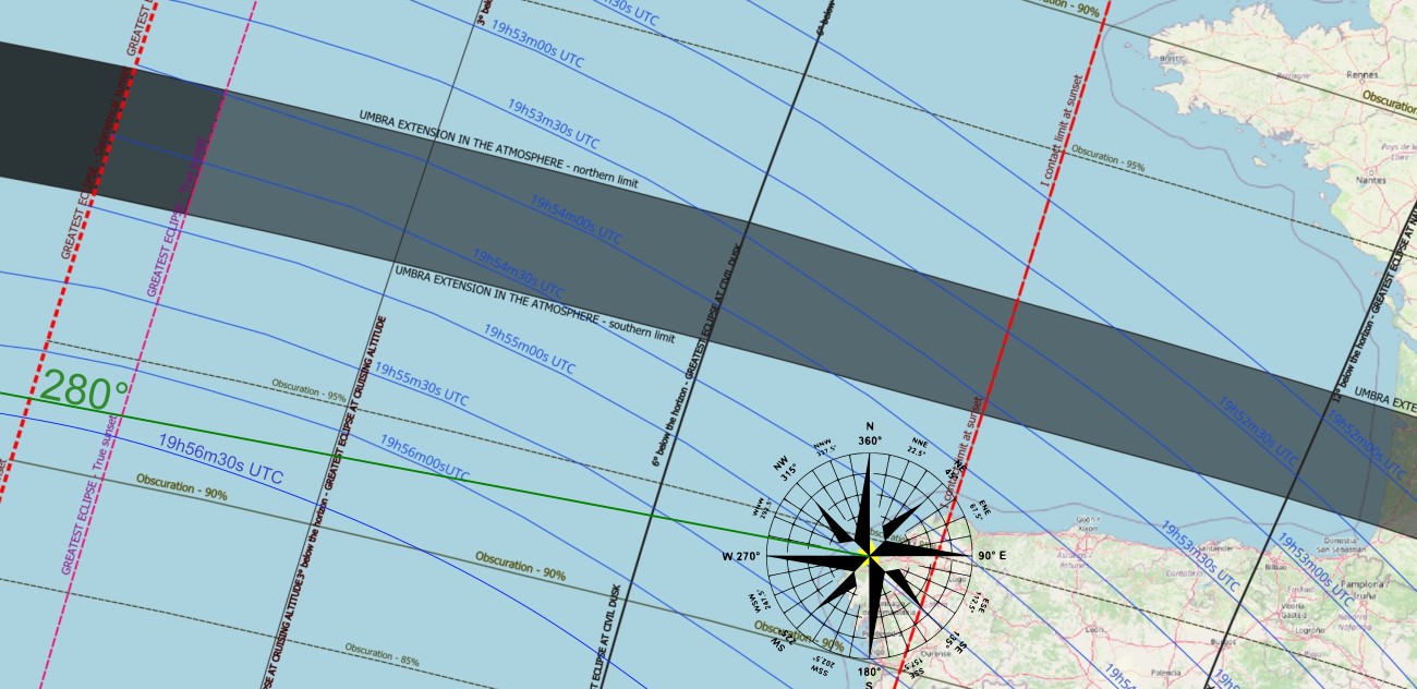
The same thing, although in a different character of complexity, would apply to the twilight standstill phenomenon. Twilight standstill, never discussed in a scientific context, marks the moment when the level of brightness remains the same despite changes in solar depression. The chart above (Pic. 91) shows the aftermath of a deep partial eclipse impact on twilight, which, by progressing in reverse sequence, allows more sunlight to penetrate the atmosphere. On the other hand, as the Sun goes deeper beneath the horizon, the amount of light decreases. The illustration below should help you understand this phenomenon (Pic. 92). The “standstill” marks the period when these two factors equalize the level of light. However, the explanation of this phenomenon should be done carefully, as the device results show it only at the given azimuth! Essentially, the twilight standstill should apply to the general level of light observed or measured on the scene during the eclipse. In other words, it should be a result of the amount of light coming from various sections of the sky. If we want to measure it globally, a very precise Luxmeter would be required, with some neutral orientation, which would clearly report how the light level changes in a holistic sense. Moreover, the whole discussion applies to the azimuth only, but the device was oriented at an altitude of approximately 30° above the horizon. The slant range computations would need to be used for more detailed results, although for general purposes, they can be omitted.

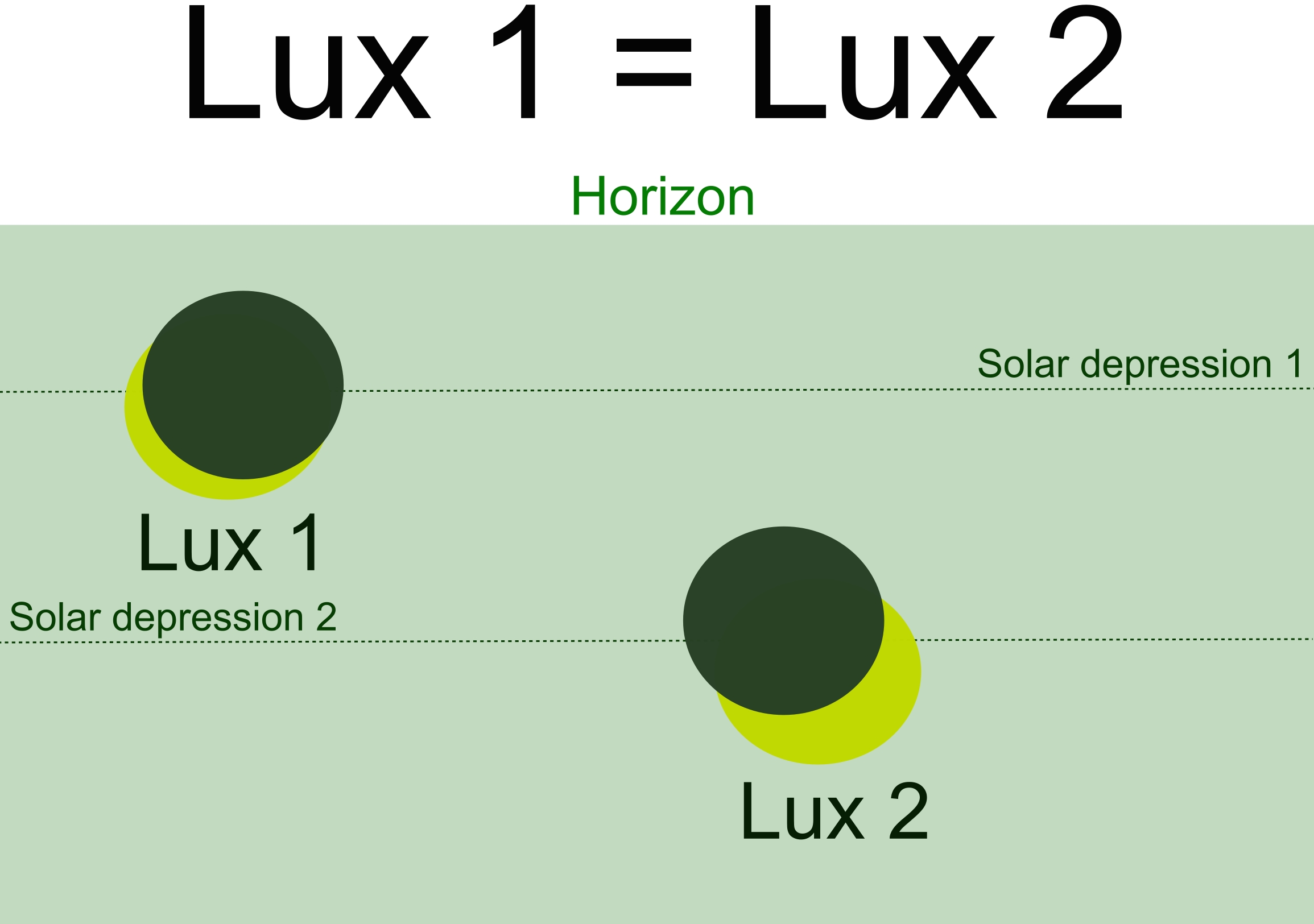
The increasing cloudiness from the northwestern direction featured separated blocks of clouds, allowing the observer to see small gaps just above the horizon. Even if the sky was clear enough outside of the estimated extension of totality, the extinction of light was pretty noticeable. At the beginning of twilight, the horizon featured enhanced reddening caused by a high level of humidity, which negatively influenced the degree of atmosphere clarity (Pic. 94). This situation persisted over the entire eclipse event, as the light scattered by the lowest layer. Thereby, the light coming from the farthest sections of the sky was attenuated by thin water vapour droplets. We must know that the planetary boundary layer, which is the lowest and, therefore, the densest, contributes most to the light scattering and extinction.

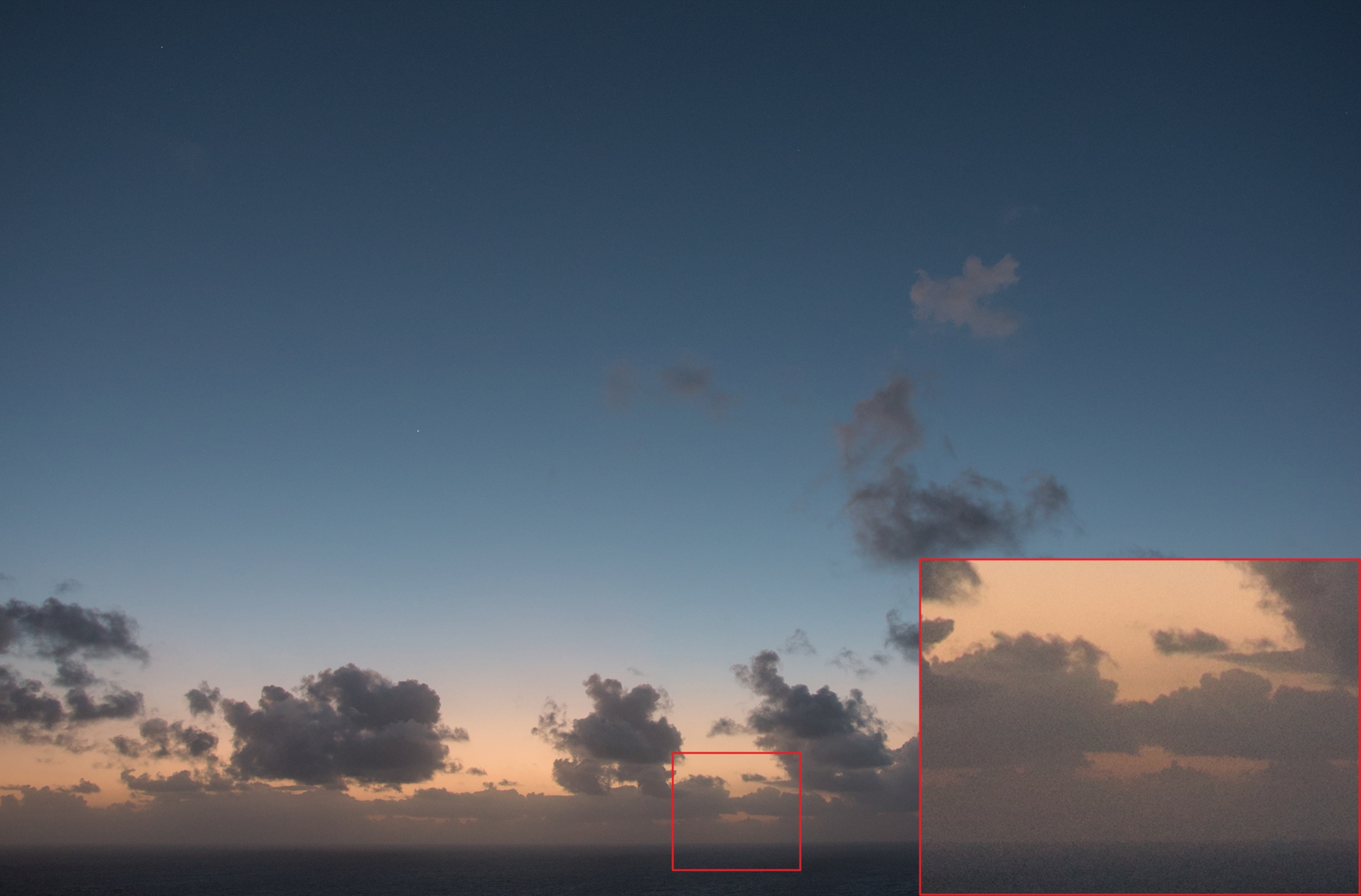
Despite a multitude of extended gaps between the cloud blocks visible at the horizon, there are not many details visible there, as everything just above the horizon is placed within the absorptivity, defined by the Beer-Lambert Law, about which some discussions were conducted in this article. The level of detail within this section decreased as the level of scattered light decreased due to the eclipse’s progress. The farthest section of the sky shows quite well how the circumstances changed as the eclipse progressed. The sequence of shots below includes several crucial moments, at which an observer can see between the clouds an apparently bright sky with an intense reddish tinge, which gradually diminishes as they move their sight away from the solar azimuth towards the north. Next, the gaps are gone and merged with clouds due to a small level of scattered light. The sky brightness at the northwestern azimuth wasn’t bright enough to let any scattered light reach an observer’s eye. The weak light, significantly reduced by the presence of the umbra, was scattered away within the planetary boundary layer.

There were passing rainfalls observed in places, but rather as isolated virgas, which haven’t interrupted the phenomenon in general. The gaps reappeared shortly after the umbra left that direction. It was a good example of the Beer-Lambert law in low-light conditions. This law states that the absorbance of light by a solution is directly proportional to the concentration of the absorbing substance and the path length through which the light travels. That was quite a clear evening after passing a cold front. All the water vapour droplets combined with a relatively small aerosol concentration contributed as a medium in which the indirect intensity of sunlight was decreasing.  We can assume that this medium, known as the planetary boundary layer, was homogeneous and plane-parallel. Even so, the conditions of light attenuation were quite specific, as the source of indirect light wasn’t uniform. The picture below shows various circumstances of light attenuation across nearly 90° of the horizon, where the eclipse occurred. The brightest section was observed just left of the approximate solar azimuth, where the amount of scattered sunlight was significant enough to be dissipated on water vapour particles and aerosols within the planetary boundary layer. The farthest cloud bands look less dark than the closest ones, which is typical for the Beer-Lambert law. The adjacent sections look darker, and the gaps between the clouds are less visible. They’re almost gone within the shadowed primary twilight sky and visible again north of this section against the clouds engulfed in total eclipse darkness.

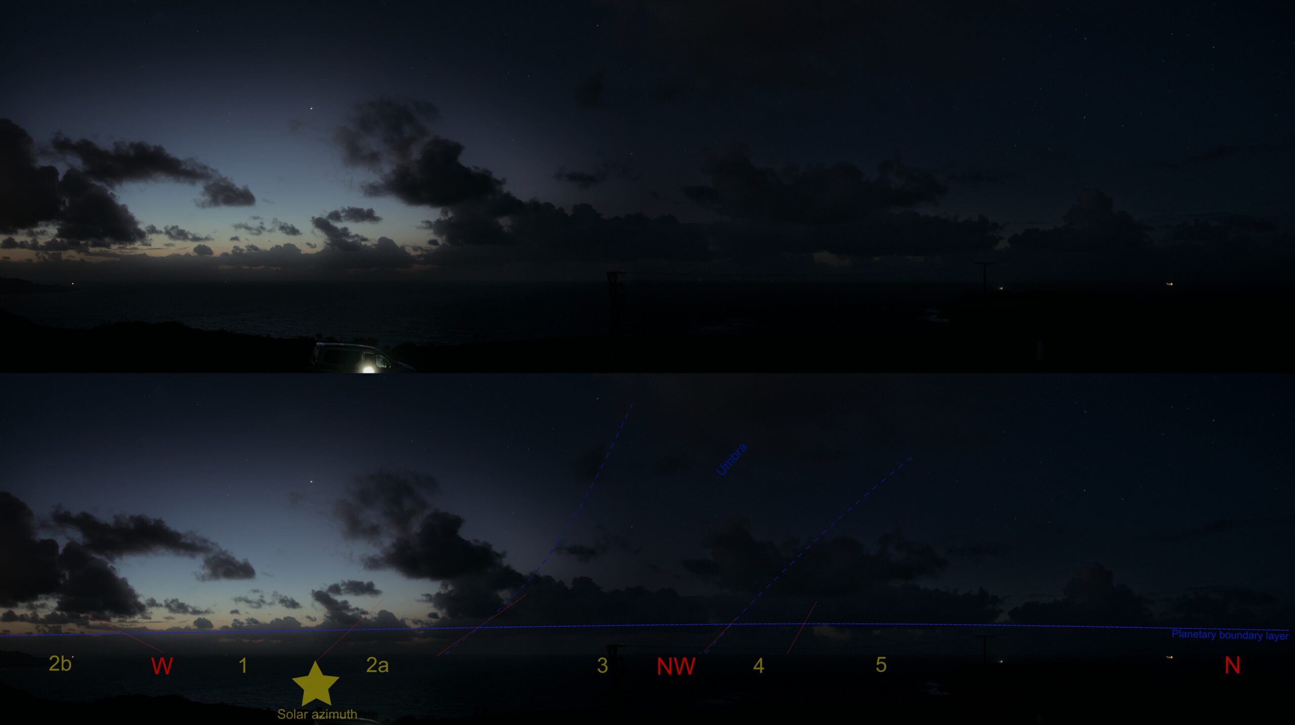
The western direction, which was the brightest, revealed how the indirect sunlight was scattered away. The clear gaps below the blue line are significantly darker in all the cases, or are not even visible within the shadowed section of the sky. The dimly lit atmosphere behaves analogously to a typical celestial object, which is simply not visible just above the horizon due to extinction. The way the light would be scattered without the influence of the planetary boundary layer, which is technically visible just above the blue line, leads to an understanding of the Chapman function. This function explains the evaluation of light attenuation along the rays of grazing incidence in a spherical atmosphere. It is defined as a factor by which the normal optical thickness above the point of observation has to be multiplied to get the optical thickness or the attenuation along a slant ray. (Sekera, 1968). The Chapman function describes how much of the solar beams is absorbed by the atmosphere at various altitudes. In contrast to Beer-Lambert light scattering, it takes into account the curvature of the Earth’s atmosphere and the slant path of solar beams. At twilight, when the Sun shines from below the horizon, the solar beams pass through the Earth’s atmosphere at various altitudes. The result is observed in multiple colorations of the twilight sky. As the sunlight travels slantwise through the Earth’s atmosphere around sunrise and sunset, the amount of absorption depends not only on the vertical thickness of the atmosphere, but also on the slant path length that the sunlight travels. During twilight, sunlight penetrates the Earth’s atmosphere, while the ground is already in shadow. Next, the atmosphere becomes plunged in Earth’s shadow as the twilight progresses and the spherical Champan function can be applied, as it considers the Earth’s curvature. Even if the Sun is below the horizon, solar beams can still pass through the atmosphere, as illustrated below (Pic. 95).

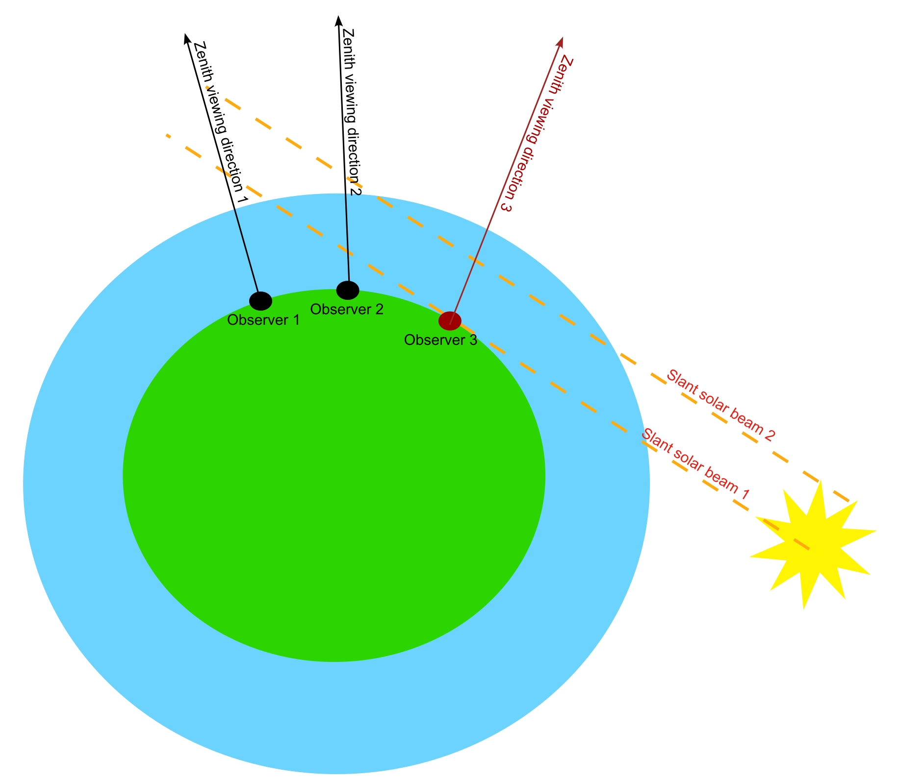
For observers in Spain during the greatest eclipse impact on twilight, the solar zenith angle was between 98° and 99°. That means that the moment at which the slant path of solar beam 1 grazed the lowest Earth atmosphere wasn’t geometrically visible. Technically, at the horizon, an observer could see the same solar beam path, which penetrated at least the lower stratosphere, so that its way through the atmosphere was longer than observed from the perspective of sunset. As we know, the solar beam at sunset travels 38 times longer through the atmosphere than it does from zenith. In this situation, the same solar beam doesn’t stop at the terminator line, but travels further, penetrating the Earth’s atmosphere in reverse sequence until it eventually leaves it. It explains away the intensive reddening of the horizon and the quick transition into other coloration of the sky as the altitude above the horizon increases. Imagine the slant path of another solar beam, like solar beam 2, which penetrates the upper atmosphere. There, due to a slight decrease in density, mostly short light wavelengths are scattered, giving the upper sky a blue coloration. That’s why during twilight we never observe the entire red sky, but only its lowest part near the horizon. Of course, the sky might have some reddish tinges, which have already been discussed throughout this entire article.

10. OTHER LOCATIONS

There are not many reports of partial solar eclipse observations over Europe or their impact on twilight. According to the Wikipedia article, the only area from which the eclipse observations were successful was Scotland. Despite a good visibility of a partial solar eclipse over the British Isles, bad weather interrupted the event. I couldn’t find anything in South Iceland, where the weather was good enough. The same would apply to any location at which the eclipse occurred that day. Potentially, there are some reports on various Facebook groups that I haven’t had the opportunity to review due to the vast amount of reports from America.

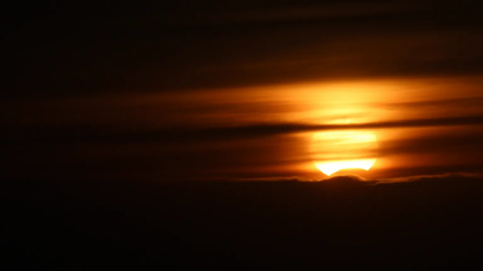
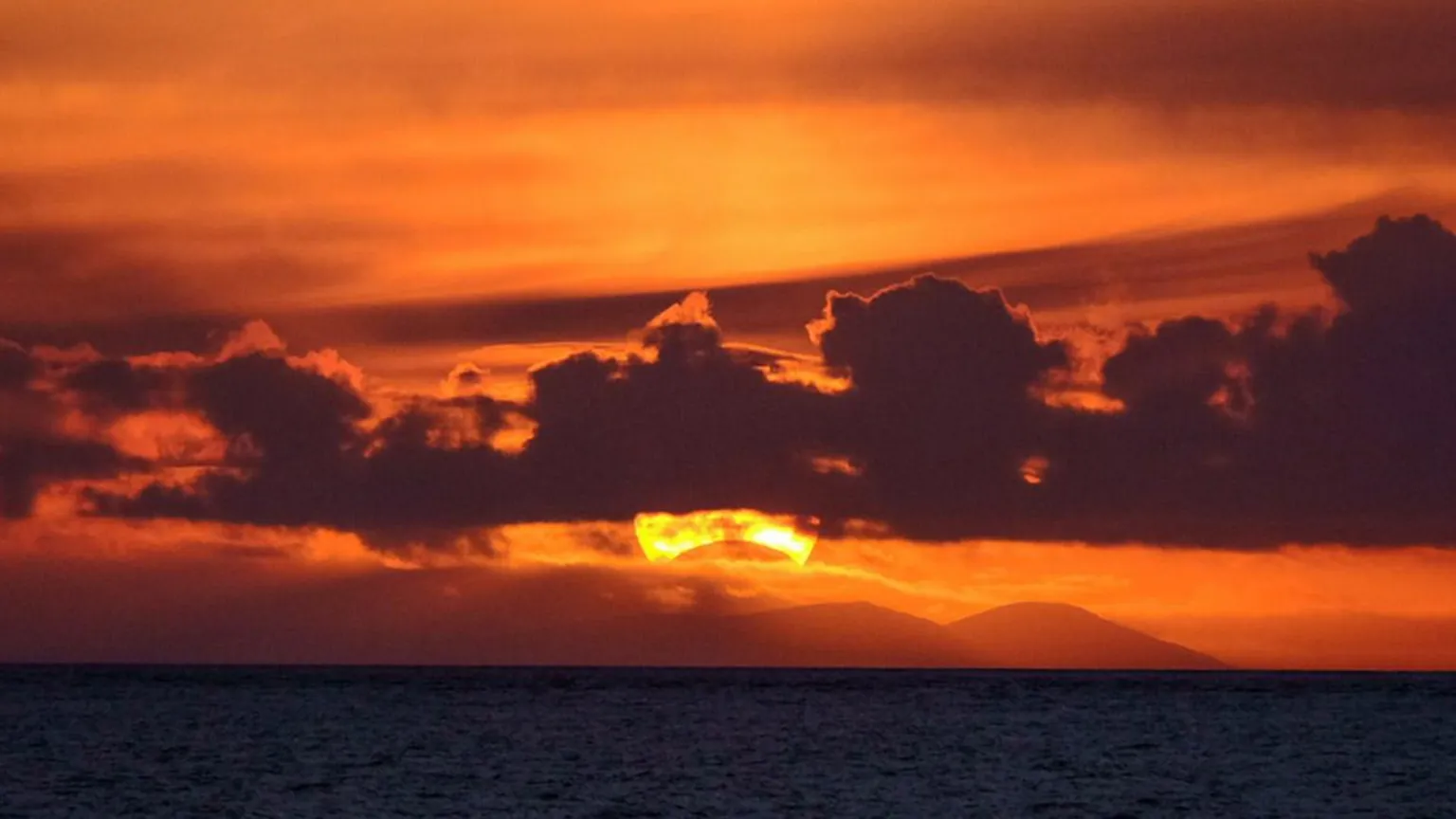
Interesting, although not so curious as in Spain, was the impact of the solar eclipse on twilight in Western Europe, which unfortunately hasn’t been observed by anyone. However, the phenomenon was detected by high-resolution webcams located in western Germany, which, despite the poor weather, were able to show the difference in sky brightness in the elongated gaps between the clouds (Pic. 99)

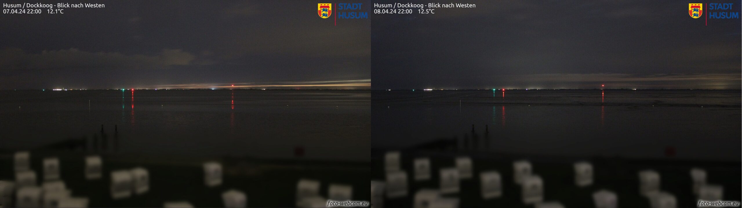
Despite small magnitude and obscuration, the eclipse impact is significant at this portion of astronomical twilight, when an observer is unable to see the sky directly illuminated by the Sun. In a practical sense, the horizon, even at the solar azimuth, isn’t discernible easily at this moment of twilight. By using a longer exposure, everything becomes visible, because the ozone layer at solar azimuth still receives a large portion of scattered light, making this section of the sky relatively bright. However, the partial solar eclipse influenced this stage of twilight quite seriously, as the horizon sky between the clouds features very low brightness. I would guess, without any computations, that the eclipse-induced twilight in northwestern Germany corresponded to the solar depression of about 14.5 °, which marks the “true dusk” appearance. This is the first observation of solar eclipse impact on astronomical twilight, which shows an exciting situation and will require further study and observations in the future, especially under clear skies. As the lowest atmosphere up to 40km is completely shadowed, the complexity of this phenomenon is different. Moreover, the eclipse obscuration wasn’t the largest, as the culmination occurred about 15 minutes earlier at that location. Another fact is the webcam ISO sensitivity and sensor properties, discussed briefly in this article. This particular comparison shows that probably this webcam operated at very similar parameters at the same moments of twilight.

11. WEBCAM REPORTS

Aside from the on-site observation, I conducted “traditionally” the remote observation by using the leading webcam provider, Meteogalicia. The undeniable benefit of this provider is the webcam backup available for the entire day and the preceding day. As the eclipse event occurred in the evening, all the streams could be downloaded as the .mp4 files after midnight. They include the 2-3 minute time-lapses with shots taken every 2 minutes. The idea is excellent, unfortunately, these webcams don’t operate well beyond the civil twilight. At least, there is a plus side to it – they don’t fluctuate as much in terms of ISO sensitivity. As a result, it was pretty easy to detect the changes in the brightness level as the eclipse progressed. In light of the technical circumstances, only the first part of the event was detectable, without the greatest phase, because it was too dark. There are over 20 webcams across the Galicia region, but I’ve selected a few of them with a good bearing and acceptable weather conditions around the eclipse event.

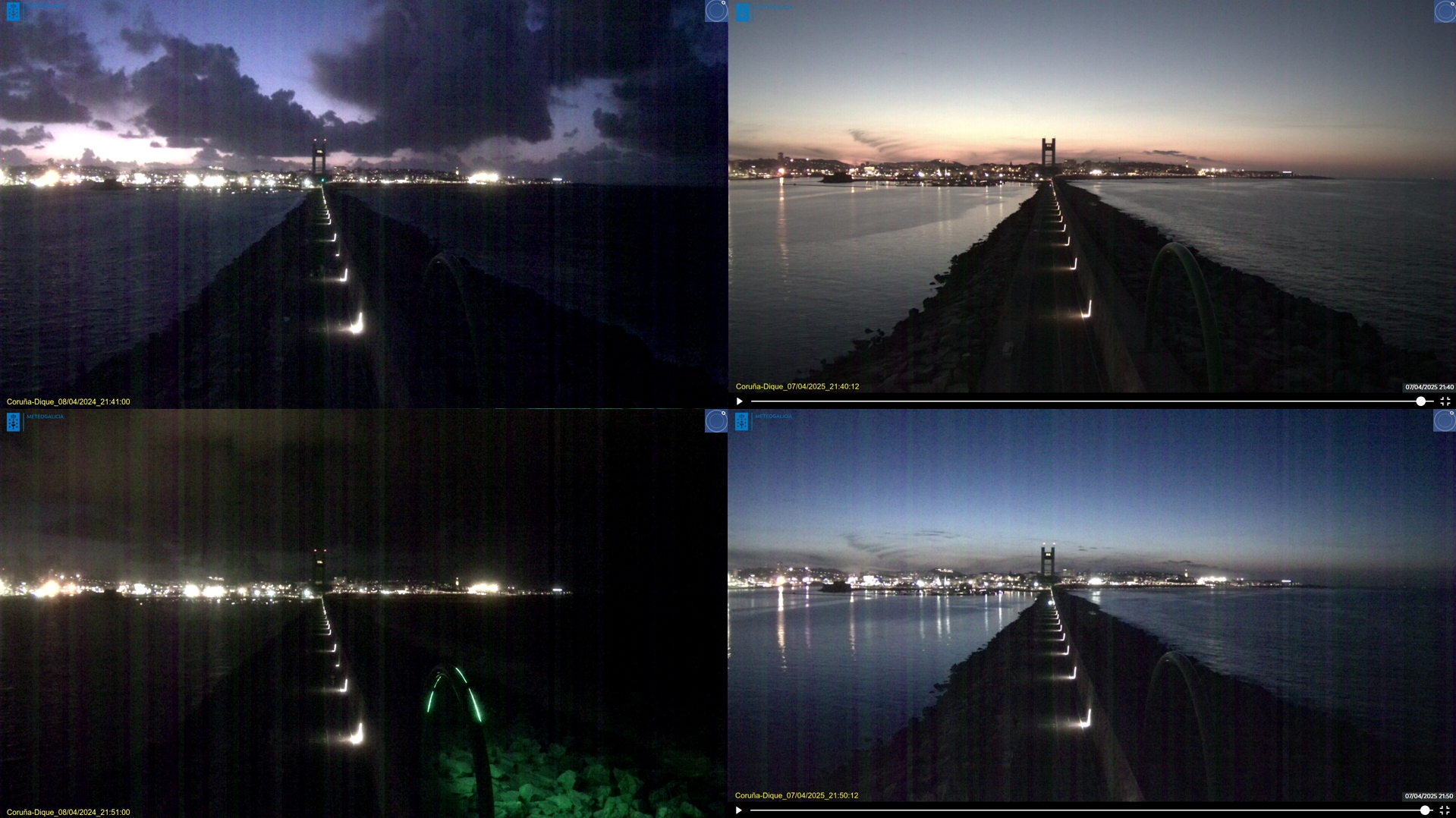
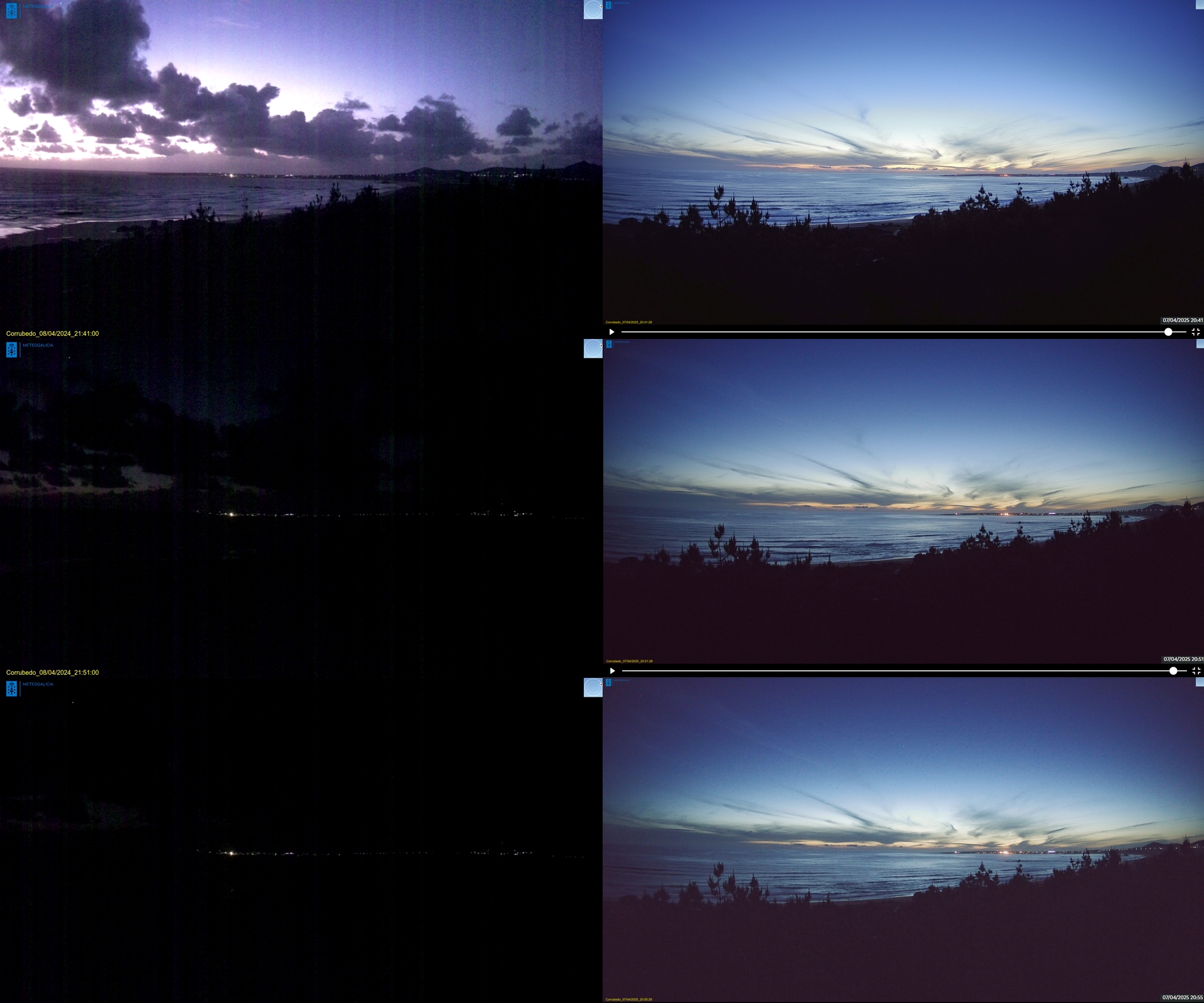
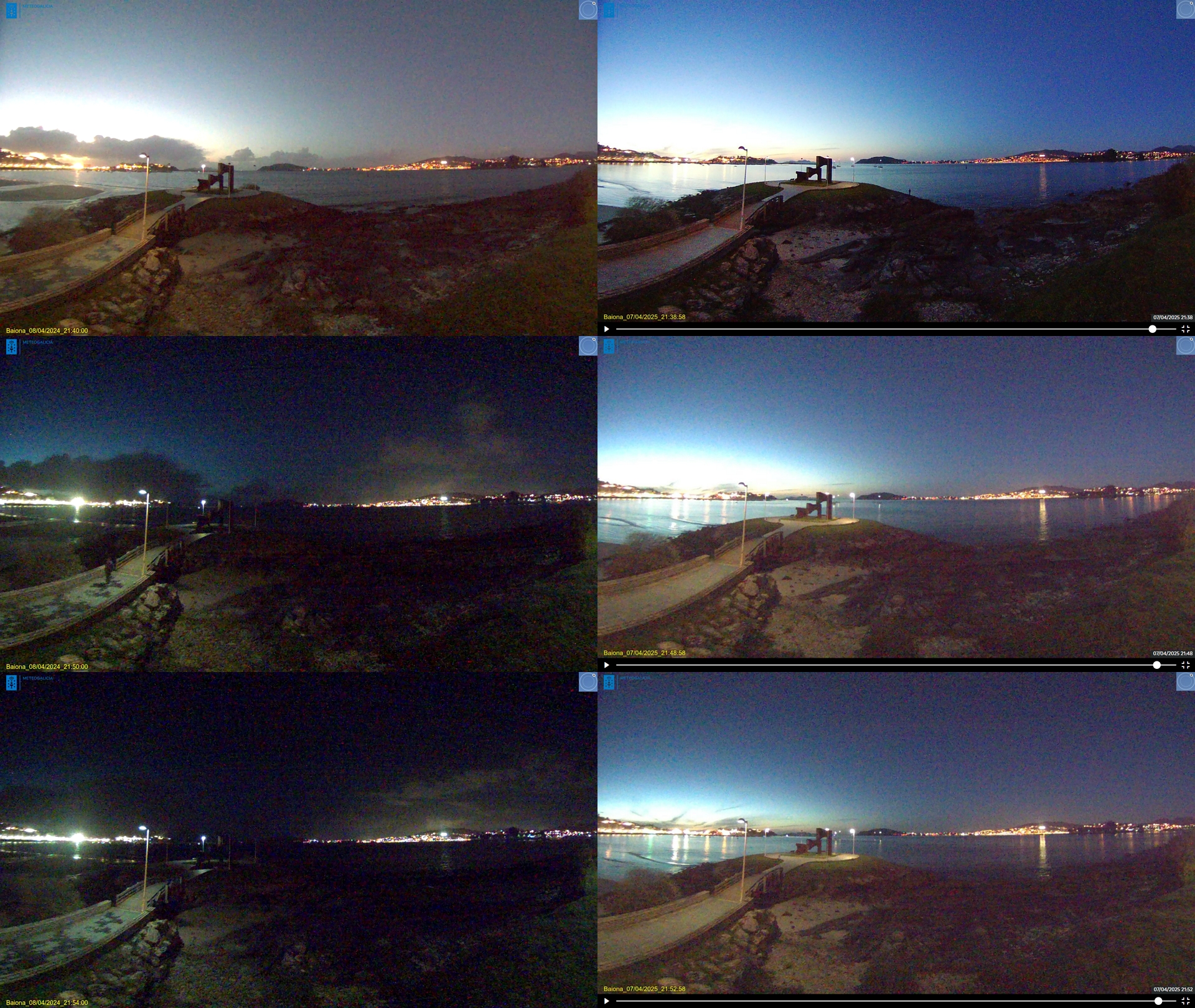
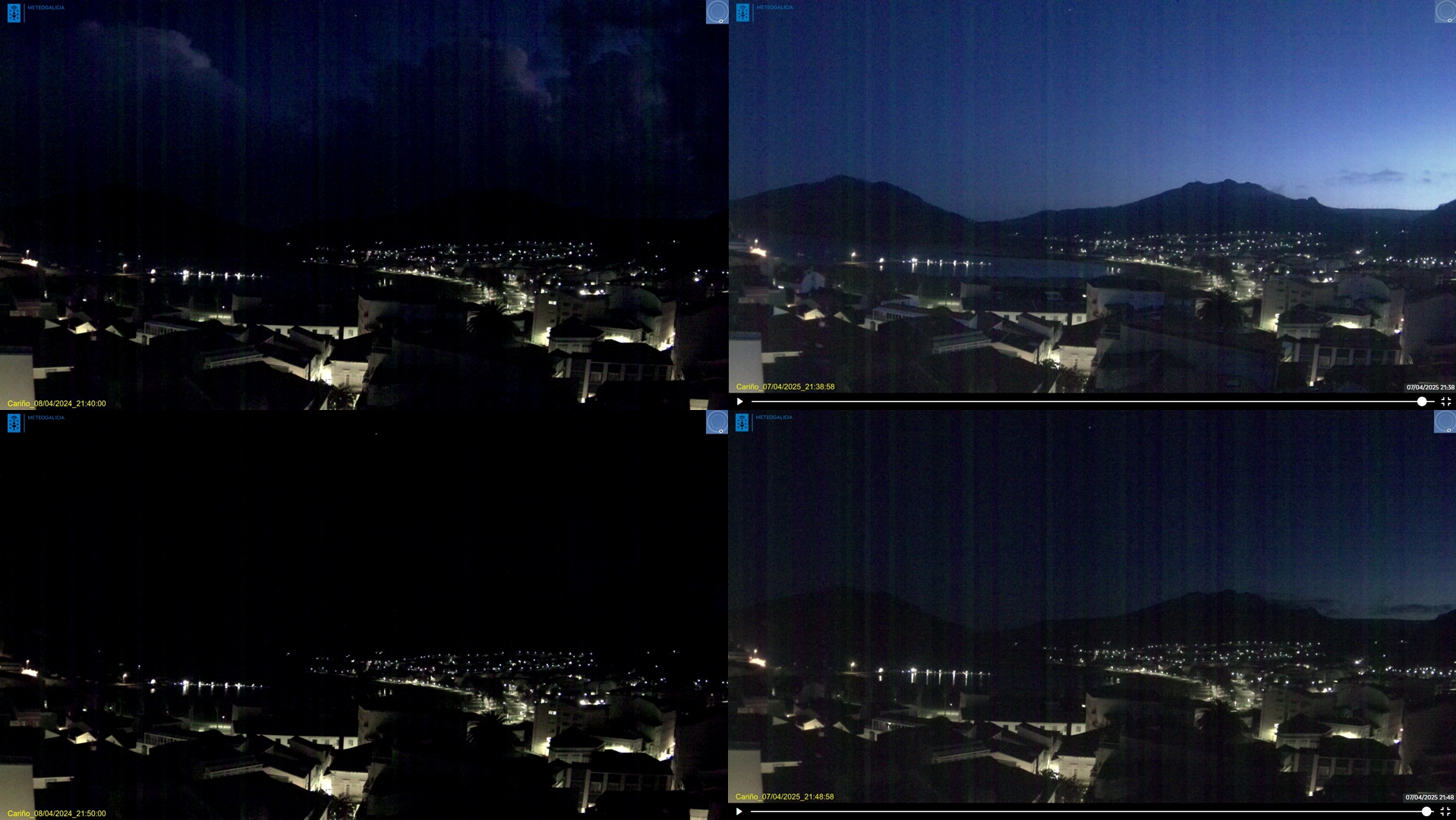
All these examples show the comparison at 21:40 and 21:50 UTC+2, where the left side depicts the eclipse-affected twilight on April 8, 2024, and the right side shows the normal twilight captured on April 7, 2025, with correction for day length if possible. The sunset on April 8 was about 1 minute later than on April 7. Due to the inappropriate weather, the reports from April 7, 2024, weren’t possible. In some locations, the moment of the eclipse culmination was captured, as the impact was weaker due to a smaller eclipse magnitude. The largest eclipse impact is visible on A Coruna (95 % of obscuration) and Cariño (96% of obscuration). The webcam orientation at Cariño was the only one headed away from solar azimuth, towards the south. The apparent difference in illumination is the smallest here. In all the cases, the cloud blocks interrupted the view and forced the cameras to change their ISO sensitivity. The best report comes from Baiona webcam, where the sky at the culmination of the eclipse was clear. The twilight glow is curved from the north (Pic. 104), which might indicate the proximity of the umbra, which wasn’t very visible from that location. When examining the twilight glow under normal conditions, it appears quite similar. It makes the report ambiguous.

It’s the best report, considering the greatest eclipse impact. This is also because of the relatively low obscuration, which allowed more light from the twilight glow to be detected by the webcam, unlike the devices recording the same event further north. This set of webcams may be more helpful in recording the 2026 total solar eclipse event in Galicia, allowing observers to analyze the event from various perspectives. The full report from random webcams, both from southern and northern Galicia, can be watched here.

12. SUMMARY & LESSON LEARNED

Twilight is an integral part of life on Earth, marking the visual transition between daylight and full darkness. There are several foundational studies on the progress of this interesting celestial phenomenon, which have led to classifying it into three distinct phases and characterizing it by variations in latitude and season due to atmospheric density. Unfortunately, there are not many publications concentrated on crucial aspects of twilight brightness. Additionally, there is an utter scarcity of work on the behavior of the Earth’s atmosphere at the edge of the solar eclipse zone. Despite just a few publications about the influence of solar eclipses on twilight, nobody has undertaken a study of this marvellous phenomenon in modern times. This article describes the first observation of solar eclipse impact on twilight in current times, characterized by easy access to digital photography, which allows observers to collect decent visual reports of this understudied phenomenon. The shortage of observational and, thereby, the scientific approaches poses a significant challenge to reporting events such as this. Another problem raised on this website is the unawareness of local people regarding the lack of local astronomical clubs or scientific institutions that could conduct similar observations in the area where the geometrical extension of the solar eclipse is expected. Moreover, it’s extremely hard to convince eclipse chasers to choose the view of eclipse-induced twilight over the solar eclipse event. This observation was a result of long-term brainstorming and a dilemma between the total solar eclipse opportunity in Texas, with nearly 4.5 m length, and its significant impact on twilight in European conditions, where the weather, by definition, is unfavourable. Another thing was the cost, as the trip to Spain was drastically cheaper than the journey to Texas. Therefore, I could bring my whole family instead of flying alone. Thankfully, the decision was perfect, as the webcam reports aren’t good enough, and in the situation of watching the totality in Texas, the twilight matter would remain unresolved.
The observation was successful due to the pragmatic decision to change the venue to a less interesting one with respect to the eclipse magnitude. It was worth losing nearly 2% of the precious eclipse culmination to make a quite clear report of the atmospheric behavior during the eclipse-affected twilight. Thanks to this, several crucial aspects could be developed and presented at the SEC 2025 at the University of Leuven. I was focused on confirming the aspects observed on previous webcam-based observations and concentrating on other accompanying events, which wouldn’t be possible to observe by the webcam. All the crucial observations and studies conducted during the production of this article contribute to the complexity of the solar eclipse’s influence on twilight, where the atmospheric behavior appears to be quite different from that observed in normal eclipse conditions when the Sun shines above the horizon. An essential aspect of investigating this behavior is understanding the peculiarity of solar eclipse geometry along the terminator line, which differs from what is typically explained to the public. The geometry of umbra behaviour around the terminator line is entirely different than on its way across the eclipse path. Some of the aspects are very similar to horizontal solar eclipses observed near sunrise or sunset. It triggers unrivalled optical response of the Earth’s atmosphere, about which further examinations with relevant measurements are essential for giving accurate explanations, especially within the fields that haven’t been entirely resolved during this expedition. I mostly mean the asymmetry in umbra limit coloration and the application of Chappuis bands in partial solar eclipse conditions. Moreover, each impact of a solar eclipse on twilight is different, just like the general eclipse event. The most desirable approach would include several observers placed within a distance of about 100km equipped with necessary instruments, which can make real-time reports in all directions. I personally dream about the cutting-edge astronomical project such as this, which would have an analog character to grouped observations of star occultations. The best occasion for an event such as this is undoubtedly the evening of August 12, 2026, when the eclipse’s impact on twilight will be observable over almost the entire Mediterranean region, providing an opportunity for multiple observations, as far as the astronomical societies are aware.
This ground-based observation opens new horizons for the study of solar eclipse-replicated phenomena, which were previously predominantly studied only within the daylight zone. Because the Earth has an atmosphere, the majority of them don’t stop at the terminator line, they tend to continue beyond. The specific interest could be put into the following aspects:
– influence of solar eclipse on the ionosphere beyond its geometrical path,
– vertical temperature gradient in solar photosphere (based on limb darkening effect),
– changes of weather conditions in the direct vicinity of the terminator line,
– ground-based observations of the solar F-corona,
– behaviour of wildlifr,m which the day-to-day routine is disturbed by changes in twilight,
– the interaction between the Moon and solar wind with respect to possible aurora appearance within the extended zone of solar eclipse,
– determination of the relativistic light deflection
– tourist response to the solar eclipse event with comparison to the area just beyond the geometrical path
The next most important step is to raise awareness among local observers who live within the path extension and can perform the observation without leaving their homes.
We can’t forget about the weather conditions. Due to unfavorable weather, I gained some on-site experience by chasing the clearest skies possible. The article also explains how the weather forecast works and how to interpret satellite imagery effectively. The next step will be to establish guidelines for distinguishing cloud types from satellite imagery.
Ultimately, the “lesson learned” section is reserved. Despite vast cussess of this observation, there are still things to work through. The biggest downside of this observation was the lack of fixed image stabilization, which excluded the preparation of correct animation (Pic. 105).

The solar eclipse is an elusive event that requires automation if we want to have our images fixed in one direction. This observation was, fortunately, relatively easy, as the view was concentrated pretty much in one direction. However, I wish I could have another camera with a wide-lens mount. The August 12, 2026, observation will be more demanding in this regard. Another thing is the belated kick-off of the observation. I should have started the measurements and sequences already at the 1^st contact around 21:05 UTC. I was late, as I started around 15 minutes later due to crowds. It’s not that nothing happens at this stage of the eclipse; any, even minor changes, are valuable. The third thing was lack of the laptop screen coverage, which eventually produced flares on some images headed west. When we perform optical-related reports, they can lead to a false interpretation of some celestial events.
In conclusion, I would summarize it as an excellent observation, and I hope it opens new horizons for investigations of solar eclipse-related phenomena.

ACKNOWLEDGMENTS

I want to express my sincere gratitude to the Stellarium Development Team, led by G. Zotti and A. Wolf. This research has been partially conducted using the ShowMySky mode, without which the visualization and comparison of the eclipse event between various locations wouldn’t be possible. The Stellarium software is the best simulated sky for open-source environments. With the ShowMySky mode applied, Stellarium is the best software for rendering a realistic sky in 3D, just like what you can see with the naked eye, binoculars, or a telescope. I am very grateful for the Stellarium Development Team, which, in the development of Earth’s atmosphere visualization, included the option for solar eclipse simulation. The team has already set up a vast milestone in the investigation of the impact of the solar eclipse on twilight. The scarcity of occasions to observe these events can be fulfilled by using this fantastic ShowMySky mode feature, which renders the eclipse-induced twilight for any circumstances at various solar depressions. Some forthcoming works will be based on the Stellarium ShowMySky solar eclipse simulations. I would also like to express my deep hope that, in the near future, the Show My Sky mode will be equipped with aurorae and noctilucent clouds, leading to excellent visualizations of these celestial events that coincide with the eclipse circumstances. Another gratitude I would like to express to Vladimir Romanyuk, who developed another fantastic sky simulator – the Space Engine. With version 0.99 an user can simulate the solar eclipse views from various spatial perspectives including random altitudes above the ground.
I would also like to thank Mateusz Kalisz, the leader of the AstroLife programme, who explained where to find the ShowMySky mode in Stellarium 0.23, and my family for their support during the entire trip.

References:

1. Adams C.N, Plass G.N., Kattawar G.W., 1974, The influence of ozone and aerosols on the brightness and color of the twilight sky, (in:) Journal of the Atmospheric Sciences, i. 34, p. 1662-1664.
2. Barentine J.C., 2021, Night Sky Brightness Measurement, Quality Assessment and Monitoring, (in:) Springer Natore 2021 LateX template
3. Belikov Y.E., 1996, Modelling of the twilight sky brightness using a numerical solution of the radiation transfer equation, (in:) Journal of Atmospheric and Terrestrial Physics, vol. 58, i.16, p.1843-1848.
4. Blättner W. G., et al., 1974, Monte Carlo Studies of the Sky Radiation at Twilight, (in:) Applied Optics, vol. 13, i. 3, p. 534-547
5. Dave J.V., Ramanathan K.R., 1955, On the intensity and polarisation of the light from the sky during twilight, (in:) F.A.Sc
6. Geyer E.H., Hoffman M., Volland H., 1994, Influence of solar eclipse on twilight, (in:) Applied Optics, 33(21), 4614-9
7. Green A.E. S., Martin J.D., 1966, A generalized Chapman function, (in:) The Middle Ultraviolet: Its Science and Technology. Part of the Wiley Series in Pure and Applied Optics. Edited by A. E. S. Green. Published by John Wiley & Sons, Inc., New York
8. Haber J., Magnor M., Seidel H-P., 2005, Physically based simulations of twilight phenomena, (in:) ACM Transactions on Graphics 24 (4)
9. Hulburt E.O., 1953, Explanation of the Brightness and Color of the Sky, Particularly the Twilight Sky, (in:) Journal of the Optical Society of America, vol.43, no.2
10. Jingyluan I, et al., 2024, The Responses of Ozone to the Solar Eclipse on the 21st of June 2020 in the Mesosphere and Upper Stratosphere, (in:) Remote Sensing 16 (1)
11. Kastner S.O, 1976, Calculation of the twilight visibility function of near-sun objects, (in:) Journal of the Royal Astronomical Society of Canada, vol. 70, Aug. 1976, p. 153-168
12. Koepke P., 2001, Spectral variation of the solar radiation during an eclipse, (in:) Meteorologische Zeitschrift, vol.10, No 3, 179-186
13. Lee R. L., 2015, Measuring and modelling twilight’s Belt of Venus, (in:) Applied Optics, vol. 54, p. B194-B203
14. Lee R. L. , Meyer W., Hoeppe G., 2011, Atmospheric ozone and colors of the Antarctic twilight sky, (in:) Applied Optics, vol.50, i. 28, p. F162-F171
15. Lee R. L., Mollner D. C., 2017, Tropospheric haze and colors of the clear twilight sky, (in:) Applied Optics, vol. 56, no. 19
16. Lynch D.K., Dearborn D.S.P., Richtsmeier S.C., 2017, Antitwilight I: Structure and optics, (in:) Applied Optics, vol .56, no. 19, p.G156-G168
17. Mateshvili N., et al., 2005, Twilight sky brightness measurements as a useful tool for stratospheric aerosol investigations, (in:) Aerosols and Clouds
18. Meeus J., 1997, Mathematical Astronomy Morsels, Willmann-Bell
19. Meinel A.B., Meinel M.P., 1983, Sunset, twilights and evening skies, Cambridge University Press, Cambridge – New York
20. Mukherje L., et al., 2025, Twilight near-infrared radiometry for stratospheric aerosol layer height, (in:) Remote Sensing, 17 (12), 2071
21. Nickiforov N.G., Belokrylov R.O., Belokrylov S.V.,  2011, Model of the stellar visibility during twilight, (in:) Bulgarian Astronomical Journal
22. Richtsmeier S.C., Lynch D.K., Dearborn D.S.P., 2017, Antitwilight II: Monte Carlo simulations, (in:) Applied Optics, vol. 56, no. 19
23. Rozenberg G.V., 1966, Twilight – a study in atmospheric optics, Plenum Press, New York
24. Saito M., Iwabuchi H., Hayasaka T., 2013, Physical Explanation of Tropospheric Aerosol Effects on Twilight Sky Color Basedon Photographic Observations and Radiative Transfer Simulations, (in:) SOLA, vol. 9, p.15 – 18
25. Sekera Z., 1968, Chapman Function for an Atmosphere with a Constant Temperature Gradient, (in:) Geophysic. J. R. astr. Soc. 15, 137-145
26. Sundberg R.L., 2024, Spectral image simulation for twilight conditions, (in:) IEEE International Symposium on Geoscience and Remote Sensing (IGARSS)
27. Ugolnikov O.S., Postylyakov O.V., Maslov I.A., 2004, Effects of multiple scattering and atmospheric aerosol on the polarization of the twilight sky, (in:) Journal of Quantitative Spectroscopy and Radiative Transfer, Vol. 88, i. 1-3, p. 233-241
28. Vasylyev D., 2021, Accurate analytic approximation for the Chapman grazing incidence function, (in:) Earth, Planet and Space, v.73
29. Waldman C.H., 1988, Daylight and twilight sky radiance and terrestrial irradiance, Naval Ocean Systems Center, Titan Systems Inc, San Diego, California
30. Zhan M., et al., 2025, Variation of Mesosphere Ozone and Related Constituents During Solar Eclipse on 21 June 2020 Based on WACCM-X Simulations, (in:) JGR Space Physics
31. Zotti W., Wolf A., 2025, Stellarium 25.2 User Guide, Version 25.2-1
32. Zotti W., et al., 2020, The Simulated Sky. Stellarium for cultural astronomy research, (in:) Journal os Skyscape Archeology vol. 6, no. 2

Links:

1. Scienceworld.wolfram.com: ChapmanFunction
2. https://www.unihedron.com/projects/sqm-lu-dl/
3. https://skyandtelescope.org/astronomy-blogs/the-belt-of-venus/
4. https://www.iflscience.com/a-beautiful-belt-of-venus-will-be-visible-just-after-sunset-tomorrow-59453
5. https://inlightofnature.com/the-belt-of-venus-and-the-earths-shadow/
6. Atoptics.co.uk:Belt-of-venus/
7. Epod.usra.edu:Antitwilight colors and Belt of Venus
8. https://britastro.org/journal_contents_ite/observation-of-earths-shadow-over-antisolar-sky-during-sunset-sunrise
9. Usna.edu: Monte Carlo simulations of clear twilights in aerosol & molecular atmospheres
10. https://www.omnicalculator.com/physics/distance-to-horizon
11. https://www.vcalc.com/wiki/slant-range
12. https://www.timeanddate.com/eclipse/solar/2024-april-8
13. The celestial sphere
14. Paths of the stars
15. https://twanight.org/gallery/the-elusive-bands-of-anti-twilight/
16. https://www.spectroscopyonline.com/view/understanding-the-limits-of-the-bouguer-beer-lambert-law
17. Bbc.com: Eclipse 2024: Partial eclipse seen in Scotland as most of UK misses out
18. Independent.co.uk: Clouds plague UK spectators as millions in US witness total solar eclipse
19. Irishmirror.ie/news/irish-news/cloud-spoils-solar-eclipse-irish-32540538
20. https://www.meteogalicia.gal/web/observacion/camaras
21. https://spaceengine.org/

 

Forums:

1. https://www.cloudynights.com/topic/900012-annular-eclipse-ambient-light-wavelength-shift-due-to-limb-color/
2. https://physics.stackexchange.com/questions/700302/how-can-daylight-have-a-higher-colour-temperature-e-g-6500-k-or-d65-than-sunl
3. https://physics.stackexchange.com/questions/410633/what-are-the-average-wavelengths-and-brightnesses-of-sunlight-across-the-stages\
4. https://physics.stackexchange.com/questions/521541/why-is-there-a-blue-hour-after-the-golden-hour
5. https://chemistry.stackexchange.com/questions/111389/what-exact-color-does-ozone-gas-have
6. https://space.stackexchange.com/questions/64106/computation-slant-range-d-between-a-satellite-and-a-ground-terminal
7. https://physics.stackexchange.com/questions/338406/traveling-in-the-umbra-of-a-solar-eclipse
8. https://astronomy.stackexchange.com/questions/47265/rising-time-of-a-planet-or-a-star-and-its-correlation-with-the-angle-subtended-a

 

Github:

1. Noctilucent clouds in ShowMySky model
2. Aurora in ShowMySky model

 

Wikipedia:

1. Absorption_(electromagnetic_radiation)
2. Afterglow
3. Air_mass_(astronomy)
4. Beer-Lambert Law
5. Belt of Venus
6. Blue_hour
7. Celestial_equator
8. Chapman function
9. Chappuis_absorption
10. Declination
11. Diffuse_sky_radiation
12. Earth’s shadow
13. Equatorial_coordinate_system
14. Isophote
15. Lunar_node
16. Northern_celestial_hemisphere
17. Planetary_boundary_layer
18. Sky_brightness
19. Slant_range
20. Solar_eclipse_of_April_8,_2024
21. Southern_celestial_hemisphere

 

 

Youtube: