Total solar eclipse visualization on Google Earth, part 1
Introduction
This article presents how to visualize the total solar eclipse on the most renowned geographical tool, Google Earth. The ways of using Google Earth are various. To learn more about it you can check my previous article where I listed examples of using this amazing software. Previously I used Google Earth to generate the flood simulation.
The foregoing option to imagine the total solar eclipse in Google Earth is displayed in .kmz files for solar eclipses from 1960 to 2099 provided for the public by Xavier Jubier. Those files will draw the paths and limits of the solar eclipses across the Earth’s surface. Every solar eclipse path contains the umbral northern and southern limits of a solar eclipse (plotted in black) and the central lines (plotted in blue). All files have been synchronized with the ‘Five Millennium Canon of Solar Eclipses’ tool.
Those .kmz files don’t show you the Moon’s shadow movement. To see how would total solar eclipse occurs in your area you need to refer to the animations attached on YouTube. Usually, you are able to find many shadow movement movies about the forthcoming solar eclipse. At this moment there is much visual stuff about TSE 2017. See the examples here on the Eclipse 2017 main page.
All animations are based mainly on Michael Zeiler’s eclipse maps. On his main website, you can see probably the best-prepared eclipse maps in the World. Besides, eclipse-maps.com will tell you the story of how eclipse maps have been developed since the 17th century to the present day. However, for you, the most interesting thing probably will be a gallery for the most up-to-date eclipse maps. There are several hundred eclipse maps that are being developed with GIS software applied to millions of eclipse calculations.
Both eclipse.gfsc.nasa.gov and Xavier Jubier maps feature the ‘dynamic local circumstances predictions at the click’s location’ that is available with interactive Google Maps. That is why using Google Maps is a keynote to develop the total solar eclipse visualization for the Google Earth client.
I prepared my own way to create the total solar eclipse animation, which I would like to show in this two-piece article.
How to create?
- I would like to explain to you how to create this visualization on the 2017 eclipse example in Wyoming, USA as I did for my purpose. For the initial work, you will need to open: eclipse.gfsc.nasa.gov with the virtual path of totality centered on your area (Wyoming in this case) (pic. 1) and Scribble Maps with a new map created (pic. 2).

Pic. 1 Eclipse.gfsc.asa.gov interactive map fragment shows the path of totality in central Wyoming.
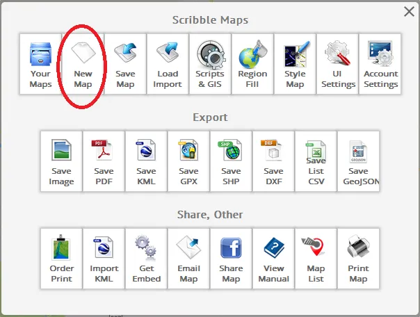
Pic. 2 A ‘New Map’ button is located on the main Scribble Maps interface (Scribblemaps.com).
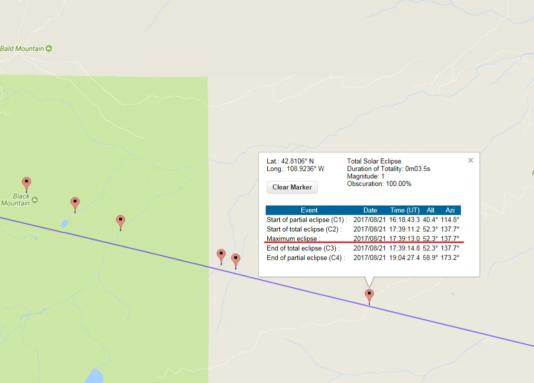
2. Click somewhere in the centerline to receive a pop-up window with eclipse circumstances. Select correctly the location when you know the coordinates of the place of your observation. On your label displayed, you have the basic solar eclipse circumstances (contacts): C1-4 with rough time (UT), altitude, and azimuth. As long as you, do not consider the Moon’s shadow moving across the sky you will not need the last 2 elements. First, you should take into account the time of 2nd contact, which will set the TSE beginning from your location (pic 3.). When you encounter half of the umbra, then refer to 3rd contact (and mid-eclipse when touching the path edge). See it later.

Pic. 3 Focus on the 2nd contact (or 3rd if you want) at the beginning when preparing the eclipse visualization.
3. Try to find the location with exactly the same moment of time for 2nd (or 3rd) contact (pic. 4 – 11) carrying on this painstaking job until you receive an umbra-looking shape on your Interactive Google Maps with eclipse circumstances. Your last point marked should be simultaneously a first point and close up the newly created shape.

Pic. 4 Carry on keeping the same time value for 2nd contact.

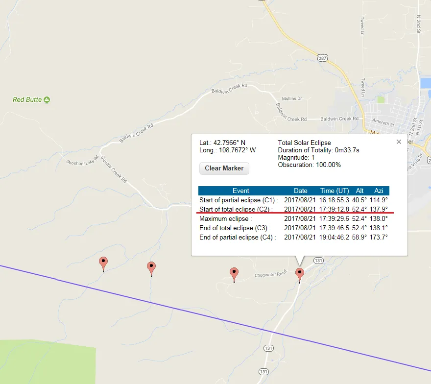
Pic. 5 Focus on the ‘Maximum Eclipse’ when touching the edge of the totality path.

Pic. 6 When you cross the place where the time of your phase touching the edge of totality (pic. 5) focus on the 3rd contact. Place your markers on recognizable spots e.g. river or road bends, lake borders, etc.

Pic. 7 We have half of the umbra 🙂
Pic. 8 Repeat the task when touching the edge of the path of totality again.
Pic. 9 When you cross the edge of the path of totality focus on the moment of 2nd contact again.

Pic. 10 There you go! Now you have traced the whole umbra.
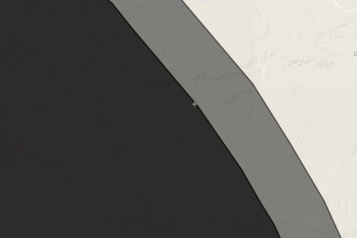
4. Go to Scribble Maps and click the ‘draw a polygon’ from the top bar. Remember also about the color adjustment, which you will find in the bottom line of your toolbar (Pic. 11). You need to adjust both lines and fills. Make it dark grey to resemble a real TSE on-the-ground reality (Pic. 12). The line thickness is not really needed, although you can make it as thin as possible setting the value “1” (Pic. 13).
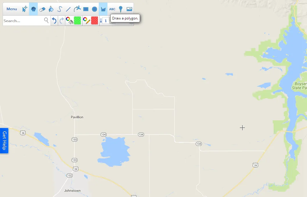
Pic. 11 The ‘Draw a polygon’ option in Scribble Maps.

Pic. 12 Select the color of both the fills and the borderlines, appropriate to the umbra conditions – black or dark grey with high opacity (60% or more).
Pic. 13 Make sure, that your line thickness is “1”. You don’t need higher values.
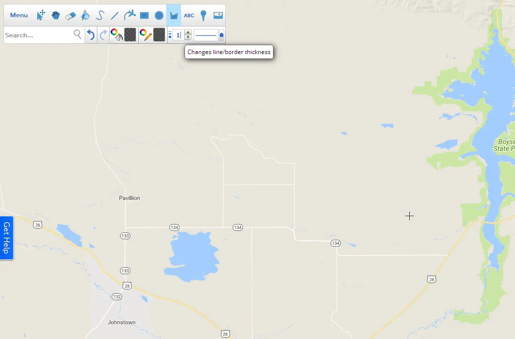
5. Make your interactive Scribble Map in exactly the same position and zoom level as the map used in the Eclipse.gfsc.nasa.gov portal (pic. 14). Try to find some clear and prominent points on both maps (pic. 14).

Pic. 14 The NASA interactive map with markers placed (above) and the Interactive map in Scribble Map with places, where the polygon border should be placed (below). Both maps in the same scale.
6. Following marked points with the same time for 2nd or 3rd contact draw an umbra-looking shape on your map (pic. 16).

Pic. 15 Umbra-looking shape borders almost ready, drawn in Scribble Maps.

Pic. 16 A ready umbra-looking shape drawn in Scribble Maps.
7. Back to your shape mapped on Eclipse.gfsc.nasa.gov interactive map. You need to find the southern or northern limit of your umbra shape. Next pay attention to the time of the ‘Maximum Eclipse’ (pic. 5, 8, 17) and follow this time exactly to the opposite northern or southern limit of your shape. In this way, you will create the sub-perpendicular line of the mid-eclipse inside the umbra (pic. 18). Next, create the line in Scribble Map and trace it exactly the same way.

Pic. 17 Following the ‘Maximum Eclipse’ time value you can trace the mid-eclipse moment for your umbra shape.

Pic. 18. Your traced umbra with the mid-eclipse line is ready.

Pic. 19 Your umbra-looking shape with the mid-eclipse line in Scribble Maps.
8. Create the centerline also. It should be easier because it is already drowned on the interactive map.

Pic. 20 Your ready umbra-looking shape with the mid-eclipse and centerline.
9. You can add up if you want (at least I did like this) the next umbra-looking shadow with borders extended e.g. 5 km outside in every direction. Then you will able to simulate the grazing zones also. Xavier Jubier gave a few examples of grazing zones e.g. for TSE 2008. The distance between the grazing zone limit and the umbra limit is not higher than 10 km. In this case, the main role plays the level of graze (which will be higher as we are close to the umbra limit) and lunar limb profile. If you pay strong attention to details you also can take into account the terrain declivity in the local area when it’s mountainous. Basically, the newly created grazing zone shape should be sent to the bottom (possibly you may have this option in Scribble Maps . I haven’t because I use the free version).

Pic. 21 The grazing zone border is around 5 km from the umbra edge.
Pic. 22 The grazing zone border around 5 km from the umbra edge filled up.

Pic. 23 A full umbra-looking shape with grazing zones made in Scribble Maps.
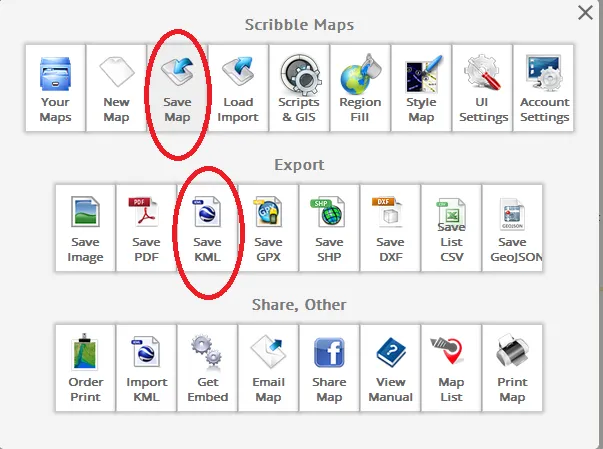
10. Now you have the first local circumstance ready! Save your map in Scribble Maps then click ‘Export KML file’ (pic. 24).
Pic. 24 First, save your map. When you have an anonymous profile remember to put a password, map name, and map ID and copy the WORKING LINK of your map to easily open it again. Next, save your map as a .kml file which enables you to see your work in the Google Earth software. I advise you to name it as a local circumstance time e.g. 11h39m13s UTC.
Now your file is ready to use in the Google Earth software! So far so good, although when you previously downloaded the eclipse path .kmz file from Xavier Jubier’s website you will see the difference in shadow location. This difference in my opinion (as a meticulous person) is quite big. The centerline and both umbra limits seem to be moved around 1,3 km south (pic. 25 – 28).


Pic. 25, 26 An inconsistency between Xavier Jubier’s .kmz eclipse path (red arrows) and eclipse.gfsc.nasa.gov interactive map causes the umbra based on the NASA interactive map to be moved south (green arrows).


Pic. 27, 28 An inconsistency between Xavier Jubier’s .kmz eclipse path and eclipse.gfsc.nasa.gov interactive map details. The umbra based on the NASA interactive map is to be moved around 1.3 km south with regard to Xavier Jubier’s .kmz eclipse path.
I don’t know where the problem is, to be honest. Possibly the problem lies in the limit of data accuracy by the departure of the moon limb from a perfectly circular figure. Another reason lies in current eclipse prediction accuracy. The Jet Propulsion Laboratory is able to calculate the Sun and Moon’s position with errors of less than 0.1 arc-second. This enables astronomers to predict the path of solar eclipses across the earth with a positional accuracy of 400 m or better (0.2 sec. of accuracy in case of contact times and duration) Unfortunately there must be something else! Because of the inconsistency between NASA’s interactive eclipse map and Xavier Jubiercounts around 1.3 km (pic. 27, 28). Probably this is the Moon’s surface topography. If we know that 1 arc second equals 1863 m at the Moon’s mean distance of 384400 km the highest features of the Moon’s limb depart from a perfectly spherical Moon by about 3 arc-seconds. However, the aforementioned inconsistency shows that the path of totality made by NASA seems to be moved around 2 km southward. The primary impact of the lunar limb profile is to introduce uncertainties of several seconds into the exact eclipse contact times and the duration of the totality of annularity. We should also know, that the centerline doesn’t show us a rough umbra diameter! It depends on the latitude and the Sun’s height during the eclipse moment.
For the sake of simplification, I adjusted my newly created umbra shape to Xavier Jubier’s eclipse .kmz map moving the whole object gradually down to plunge it within a rough path of totality.

Pic. 29 The Umbra with grazing zones ready to use. Total solar eclipse circumstance for 11:39:13 UTC, central Wyoming, USA.
Now you can enjoy your umbra for local circumstances! This Moon’s shadow is showing you what your terrain would be like during the 2nd contact! To visualize it more efficiently you can zoom in and make your view more oblique. When your place of observation is to be in a mountainous or rolling area the Google Earth 3D view enables you to see adjacent mountains also. Some of them won’t be plunged into the shadow so they will appear as much brighter objects far up on the horizon.
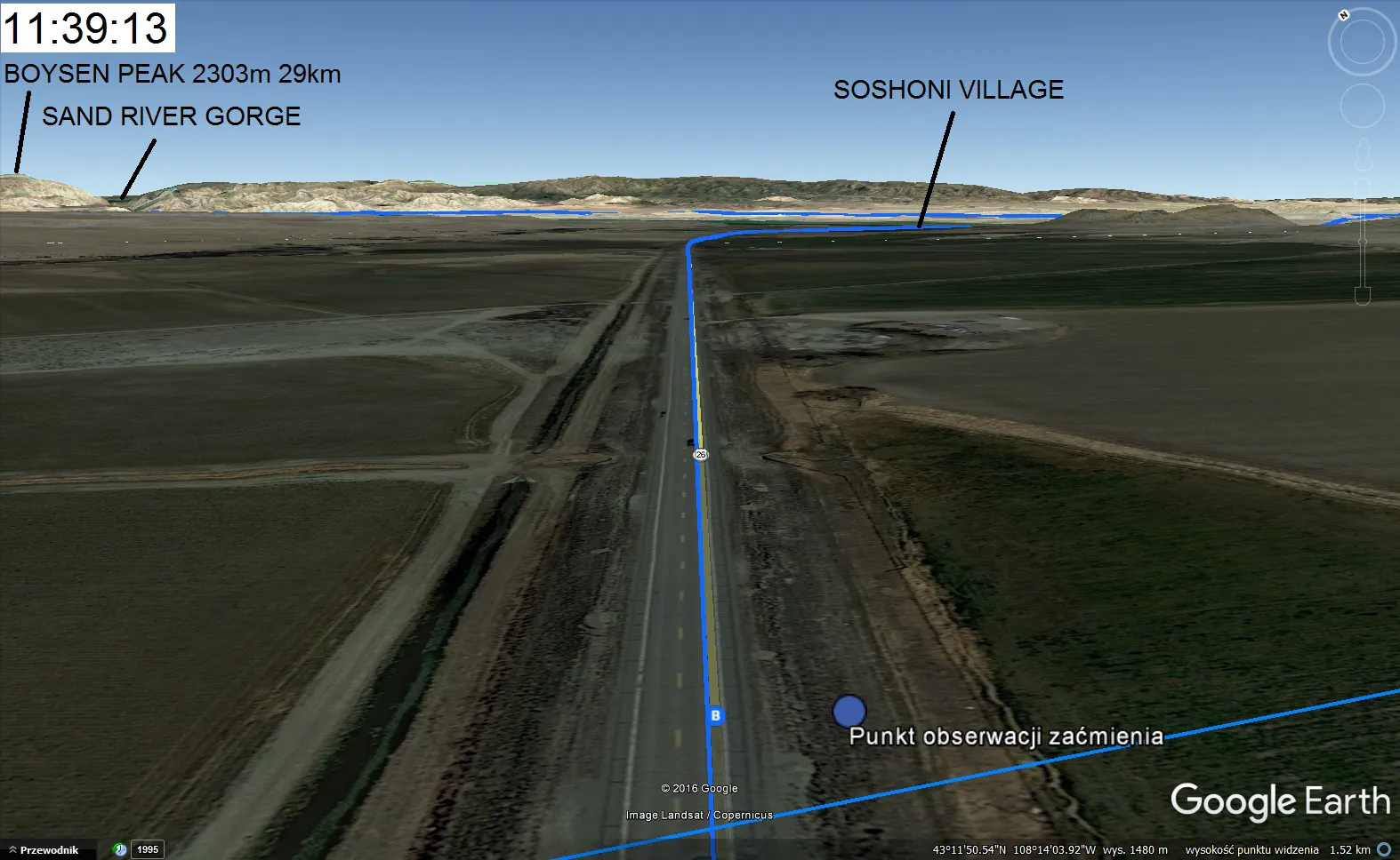
Pic. 30 A moment of 2nd contact at 11:39:13 UTC with a view towards Shoshoni village with the Owl Creek Mountains beyond seen in Google Earth just above the ground view.
The next article, which is already in production will show you how to manage the umbra-looking shape in Scribble Maps and Google Earth to make the total solar eclipse animation.
Mariusz Krukar
Links:
Michael Zeiler’s eclipse maps main page
Xavier Jubier interactive eclipse maps main page