The correct way of using QGIS Viewshed plugin

by Krukarius · 2023-06-20

Visibility analysis constitutes great importance in many fields such as sensor deployment, decisions for placement of mobile towers for maximum coverage, military operation planning, gaming, fire monitoring towers in the forest, urban design, landscape planning, etc (Saxena, Mundra, Jigyasu, 2020) or even for location graves (Lockwood, Masters, 2021). The explanations of the current text are based on long-distance observations, which are aimed at seeing the most distant possible objects from the given place. In recent years, the most recognizable tool for doing analyses such as this is available via QGIS open-source software is the Viewshed analysis plugin.
Viewshed analysis is a useful plugin for QGIS 3, which models the field of vision from a given place. The basic output of viewshed analysis is a visibility map, very similar to the viewshed layer produced by the Heywhatsthat service. The viewshed layer comes in raster format, which principle is a classification of the terrain surrounding an observation point into visible or not visible. Moreover, the plugin takes into account also terrestrial refraction, which leads to more complex visibility analysis from the specified place.
The Viewshed analysis plugin is available in the QGIS plugin repository and can be installed easily. In my opinion, the biggest problem is, that many sources explain its usage in the wrong way. Namely, the task seems to be incomplete, as the whole foundation of the issue is omitted. In this article, I will run you through the whole task step by step to make you fully equipped with the relevant knowledge needed for successful viewshed analysis in QGIS.

I. ORGANIZING THE DIGITAL ELEVATION MODEL

1. The very first element of our work should be assembling the DEM files. Because I deal with long-distance observation, I will use them even a few instead of one, presented in multiple tutorial sources. The Digital Elevation Model can be downloaded for example, from this website, but remember to set up your private account first thing. The NASA search platform looks like the below (Pic. 1),

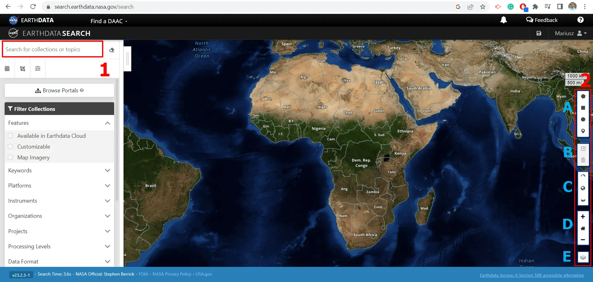
Pic. 1 The homepage of the Search.earthdata.nasa.gov service with elements important to use during this particular exercise: 1 – The search box for various topics; 2 – The navigation panel, which allows a user to search by area (A), edit searching areas or remove them (B), change the map projection (C), change the zoom level (D) or change the map canvas (E).

There are 2 bits important for you. On the left side, there is a panel with data collection, which can be filtered. Instead, it, is much better is use the search box at the top (1) and simply type the keyword of data you need. Another one is located on the right. At first glance, we would think, that it’s something like a drawing tool. In reality, we can draw the objects on the map canvas, but these drawings are for marking a certain area, which we want to get data from (2A), alternatively, they can be further edited or deleted (2B). This panel stores also the map projection options (2C), zoom level (2D), and map canvas (2E).

2. Before you start searching for DEM, let’s consider exactly which type will be the best for you. Remember, that the purpose of this article is long-distance observations, so this goal would require as much detailed data as possible in order to investigate the spots of maximum distances from where the analyzed object could be visible. The best for the time being could be SRTM 1 with a 30m resolution. The steps you should take are shown in the bound screenshots below (Pic. 2):

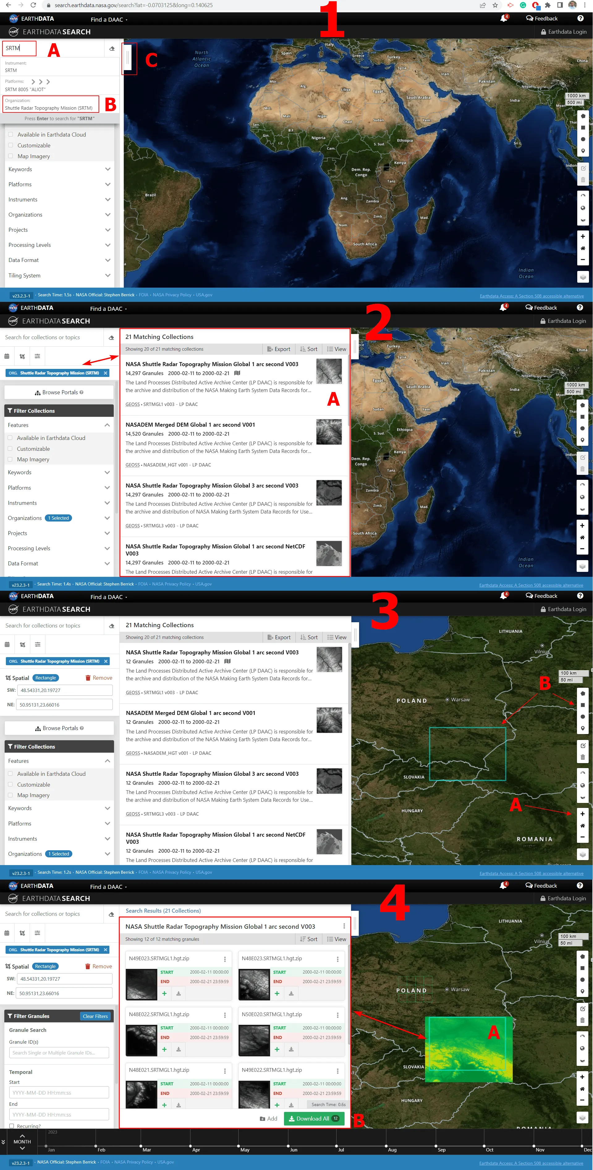
SearchEarthdata NASA gov search and download

Pic. 2 Search.earthdata.nasa.gov – the steps for searching DEM and download, where: 1A – typing the keyword in the search box; 1B – Suggested data type or organization; 1C – collapse/expand sidebar with the list of data; 2 – The data collections matching for the given keyword & organization; 3A – Changing zoom level; 3B – Drawing the spatial rectangle above the desired area; 4A – List of terrain models available for the selected area; 4B – The “Download All” option.

The simplest way will probably be typing the interesting phrase in the search box (1A) and waiting until the service lists the matching queries (1B) including the particular dataset type of organization providing them. Important is the sidebar, in which all the proposed datasets are displayed, which is visible in default mode. Because it overlays most of the map, probably you will hide it. Remember to bring it back by the button located next to the search box (1C), otherwise, you might be confused why your datasets don’t come out.
When the item (both dataset and organization) is highlighted, all the products are listed in the sidebar (2), but they are happy with the current view of the map. The default view shows pretty much Central Africa (the map center details can be found in the permalink). You can adjust the map view to the desired area by using the Zoom panel (3A) and drawing the location box (3B) or other shapes, which will indicate the exact location of your target. Once prepared, it should load automatically and you will see both the changes in the sidebar content as well as on the map, where the area bound within your drawing shape will be highlighted (4A). There is an option for downloading all of the elevation model items available (4B). They are represented by the zipped .hgt files, which are extensions of SRTM terrain models.

3. Download your data. You can do it in three ways. The first one is just one by one, in case you would like to get familiar with the particular .hgt file by looking at its preview. The second one is selective and in my opinion, it’s the best because you can decide which certain files (areas) you want to get (Pic. 3).

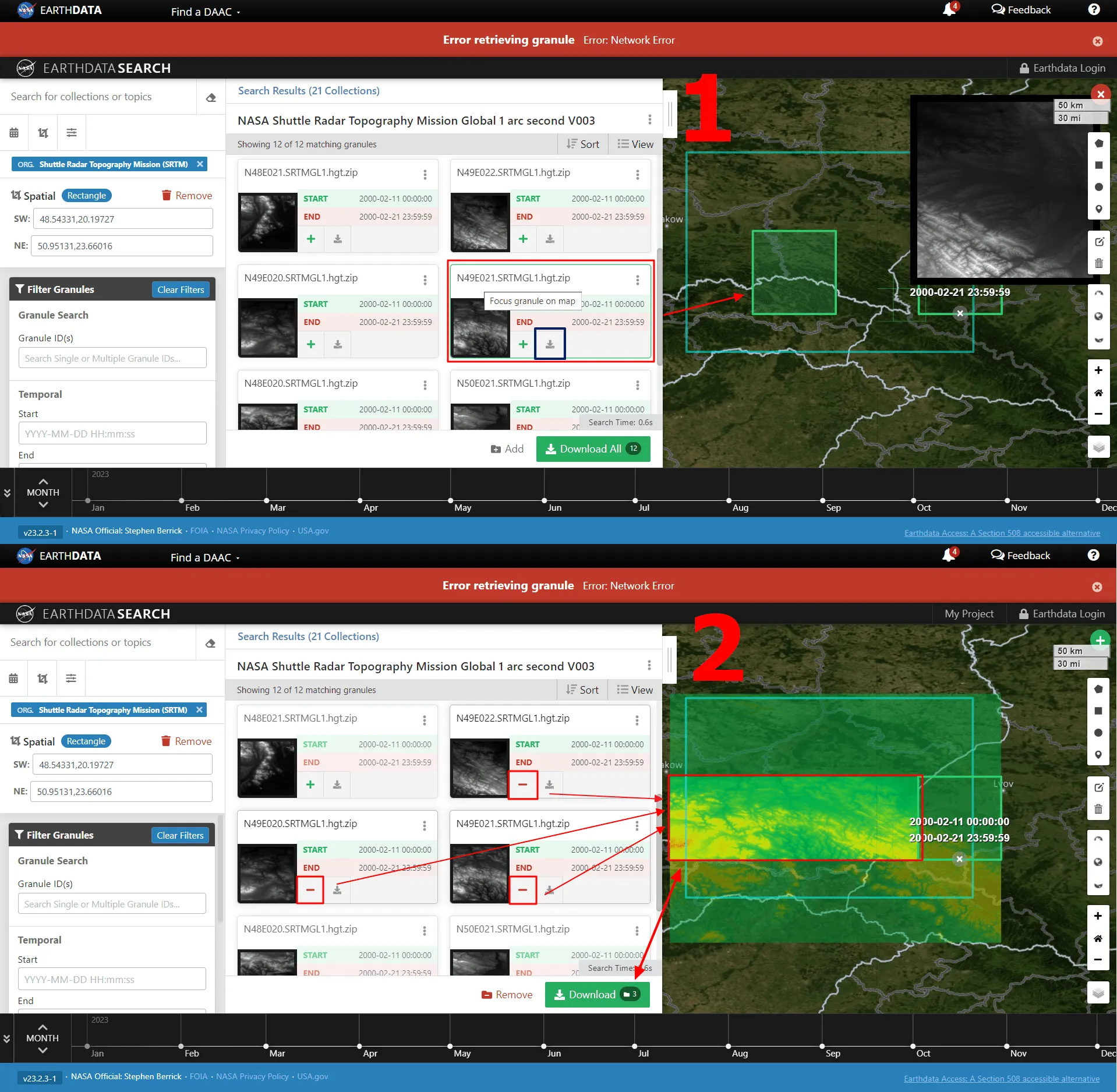
Search Earthdata NASA GOV selective SRTM download

Pic. 3 Search.earthdata.nasa.gov selective download of SRTM files, where: 1 – Highlighting the range of data within the previously selected boundaries; 2 – Selection of data prior to download.

Every single file has a thumbnail preview, in which potentially you can recognize which part of the area it shows. If you aren’t sure enough, then you can click on it and its range will appear on the map within the boundaries defined earlier (Pic. 3, 1). Next to the thumbnail you have 2 icons. One of them is the green “+” for adding them to the map (making them temporarily active), and another one is the download signature for getting them one by one as discussed a bit earlier. Once they’re selected the “+” sign turns into “–” for taking the file down just in case. Finally, the green “Download” button can be used for downloading the selected ones (2), or remove all of them by choosing the red “Remove” option just next to on the left.
In a last way, you can theoretically download them in one go, although eventually you would have to click one by one again for download without having a thumbnail and any option for insight (Pic. 4).

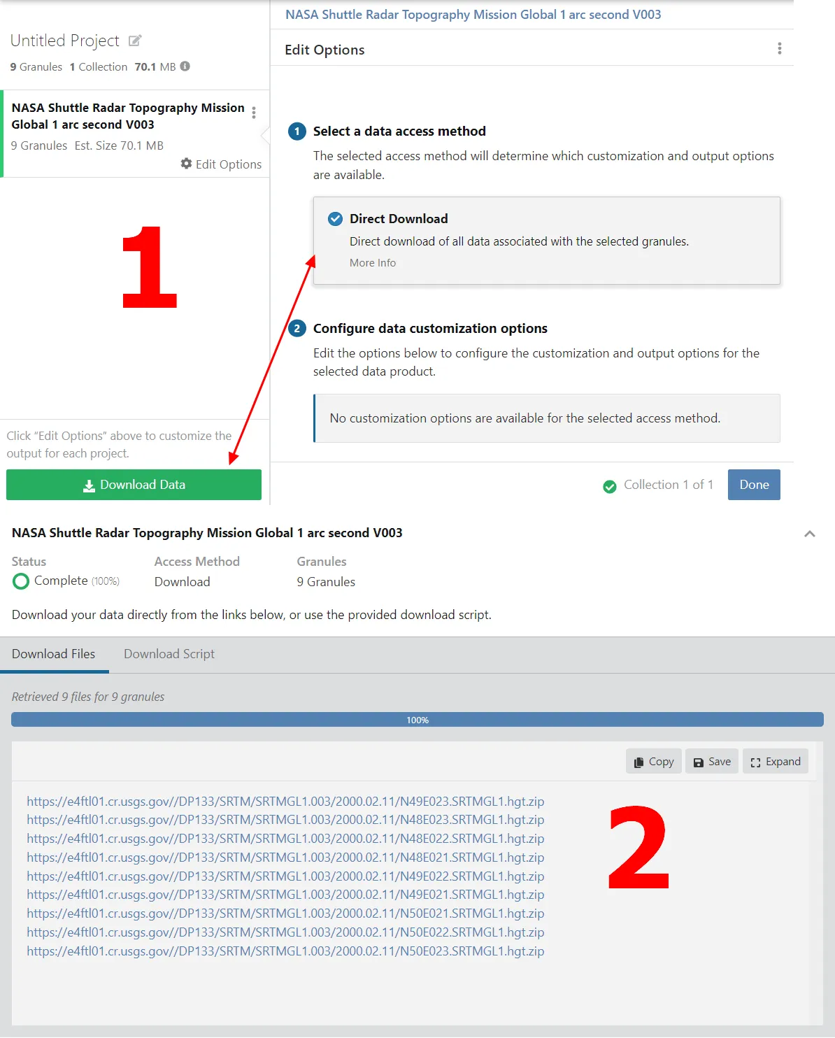
Search.Earthdata NASA.gov batch download SRTM

Pic. 4. The (theoretical) option for batch downloading the SRTM .hgt files from the Search.EarthData.NASA.gov website, where: 1 – Selection of the data access method; 2 – The list of files for download.

You can at least recognize them by the coordinates included in their names. They are named on a very similar basis to the Heywhatsthat.com visibility cloak files, about which I wrote here and I am going to text more in the near future. When the file has i.e. N49E023 in its name it means, that the box range starts at N49E23 and finishes at N50E24.

4. Unzip downloaded data. The best way is to do it in one go, although both Windows 10 and 11 don’t support this option. You can use the 7Zip application for it and follow the screenshot below (Pic. 5).

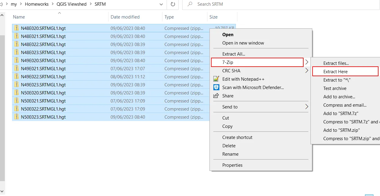
Pic. 5 Batch unzipping the SRTM .hgt files by using the 7Zip application.

By selecting 7Zip -> Extract Here you are getting all the standalone files in the same directory, where the zipped files are. As a result, the wrapped ones can be optionally removed.

5. Load .hgt files to your QGIS project. We can simply drag them to our map canvas in QGIS. They will appear as raster layers (Pic. 6).

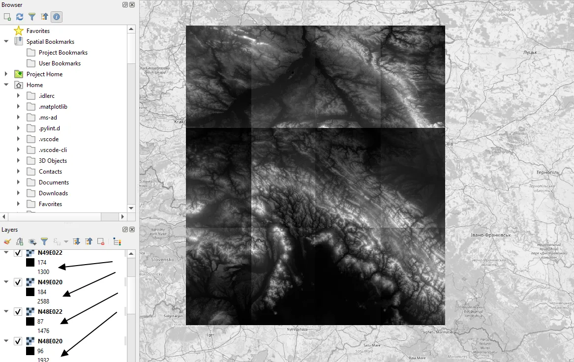
Pic. 6 The SRTM .hgt files loaded to QGIS. Look at the band ranges on every layer (file) provided.

At this stage, all the downloaded files come separately. They represent their own band range, which corresponds to the local altitude above sea level. Therefore in the layer panel, we can see the different ranges for each of the inputs. In turn, each of them has its own altitude scale. They look different on the map. At first glance, you can guess, that there are quite a lot of high mountains in the given area.

6. Merging all .hgt files it’s essential here, as we need just one big raster file with an individual color band adjusted to its altitude range. Navigate to the top main bar -> Raster -> Miscellaneous -> Merge (Pic. 7).

Pic. 7 Merging SRTM .hgt files in QGIS.

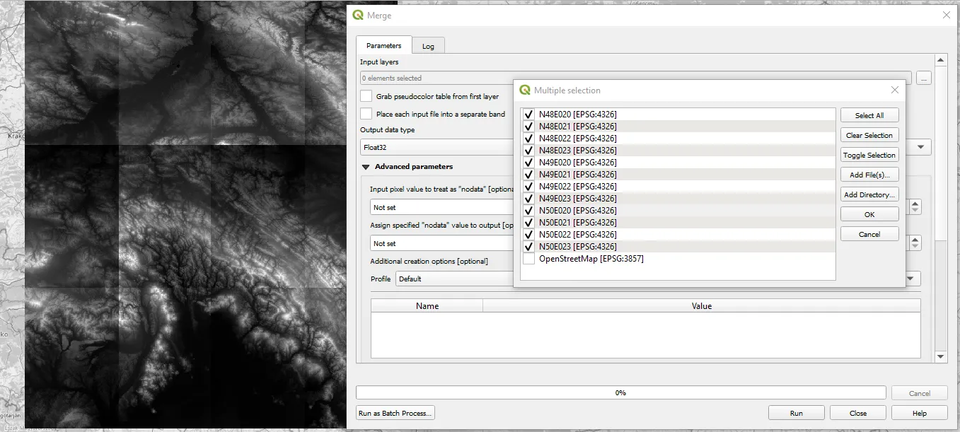
The only thing, which could draw our attention is the Output data type, which should come Float32 as default. We don’t need to change it, but just in case, we have several other options here, in which our data can come out as integer numbers. Sometimes after the merging process, you might see an error saying:

The following layers were not correctly generated

It means, that you should reinstall your QGIS or free up some space on your drive because stitching DEM rasters together might require more space than we would suppose. Alternatively, you don’t need to worry about this error, because the scratch Output file should be produced unless you want to save it to the file. Then this error might be troublesome for you.
Anyway, our final Merged layer will feature smaller contrast eventually due to a higher range of local altitude above sea level (Pic. 8).

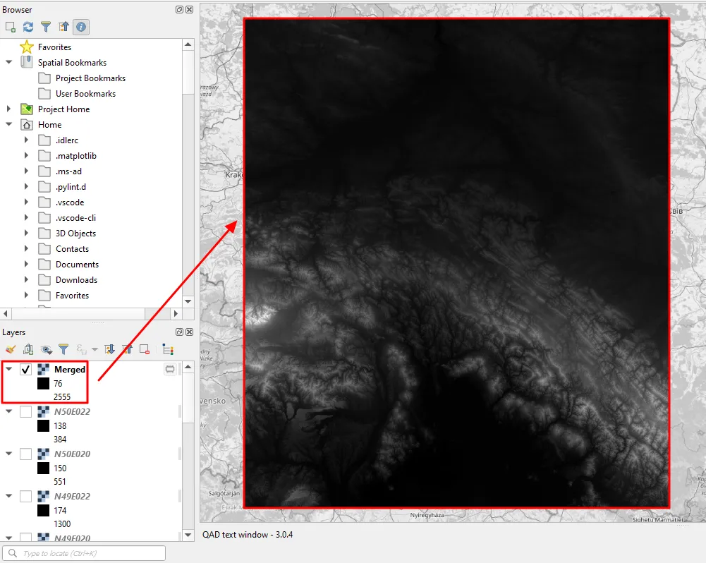
Pic. 8 Merged .hgt files into one in QGIS. The altitude range is represented in the grayscale.

Optionally you could right-click on the layer -> Properties -> Symbology and in the Band Rendering instead of Singleband gray select Hillshade or define your own color band scale by choosing. About fiddling with raster overlays you can read on this page. Moreover, it would be advisable to rename merged SRTM files to avoid further confusion across this task. Let’s call it optionally SRTM1.

7. Reproject your SRTM layer. The major reason for the reprojection is changing the CRS system from the standard one (EPSG:4326 – WGS84) to the local one, adequate for the area you are working on. Of course, you could have done it when creating (setting) your QGIS project, although if you didn’t, now it’s the right time for it.
By default, your merged raster SRTM layer probably came out in the standard CRS system, which is EPSG:4326 WGS 84. This CRS can’t be used, because its unit of measurement is in degrees. We need a unit of measurement in meters instead. For this reason, the local CRS system is required. Otherwise, you won’t be able to use the viewshed plugin due to the following error:

Raster data has to be projected in a metric system!

The most effective way of projection our raster layer is using the top Main Bar -> Raster -> Projections -> Warp (Reproject) (Pic. 9).

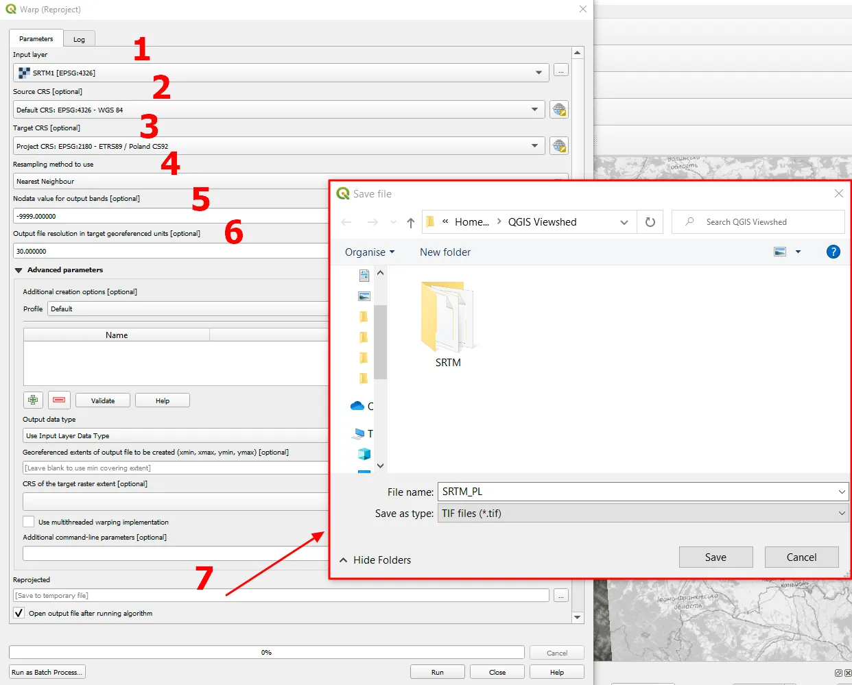
Pic. 9 Warp (Reprojection) raster layer in QGIS, where: 1 – Input raster layer; 2 – Source CRS of the input raster layer; 3 – Target CRS for the layer; 4 – Resampling method to use; 5 – Nodata value for output bands; 6 – Output file resolution in target georeference units; 7 – Reprojected file name and directory.

When the Warp (Reproject) window opens you have several fields to look at. First of all, you should select the correct raster layer (1), which will be our merged product of the .hgt files renamed SRTM1 recently. Important is defining its source CRS, which is the default one EPSG:4326 WGS 84 (2). Next, the target CRS must be specified (3), which should fit our project CRS if we want to be successful with our task. The Resampling method to use tells us about the degree of pixel conversion and represents several ways of processing, applicable for various purposes. Because we are dealing with long-distance observations, the Nearest neighbors will be the best. This option preserves the pixel values, which means, that the altitude values won’t change. In fact, the basic disadvantage of this option is, that some of the pixels might be duplicated or removed, deteriorating slightly the quality of our final output, but just a little. This method of projection is the fastest because of its simplicity.
Nodata value for output bands (5) is usually assigned to a specific numeric value to denote that data is missing or incorrect. The most frequent value here is -9999 because the projection involves rotation and scaling. Optionally you can leave this box as default (Not set) since your No Data Value is blank in the Right-click -> Properties -> Transparency -> No Data Value section (Pic. 11).
Output file resolution in target georeference units (6) must reflect the default resolution of the raster product. Since our SRTM 1 data features a 30m resolution per pixel, we should keep the 30m value in this box.
In the Reprojected box (7) we can define the name of our new raster file, save it under various raster formats (preferably .tif), or keep it as a temporary layer.
Now, our raster file is ready for Viewshed analysis!

II. PREPARING VIEWPOINTS

8. Create the point layer, in which you will store the observation location. The quickest way of doing it is to navigate to the top bar -> Layer -> Create Layer -> New Temporary Scratch Layer… (Pic. 10).

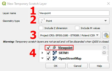
Pic. 10 Creating temporary scratch layer in QGIS, where: 1 – Layer name; 2 – Geometry type; 3 – CRS; 4 – Created layer toggled in ‘Edit mode‘ as default.

When the small box appears, provide the Layer name (1) and select the Geometry type (2). Because we are creating the place of our observation, it must be the point. Therefore our Geometry type should be the Point. Consider the correct CRS system (3), which has to correspond to your QGIS project CRS and the CRS in which the DEM file has been projected. When everything is fine, hit OK and see the new layer appearing in the layer panel (4). This temporary layer is switched to the ‘Edit mode‘ initially, so you can start working on it immediately.

9. Create the viewpoint, in other words, your observation point. If you aren’t sure enough where this point could be located, change the transparency of your raster SRTM layer in order to see the map canvas below. You can do it quickly by right-clicking on the raster file -> Properties -> Transparency (Pic. 11).

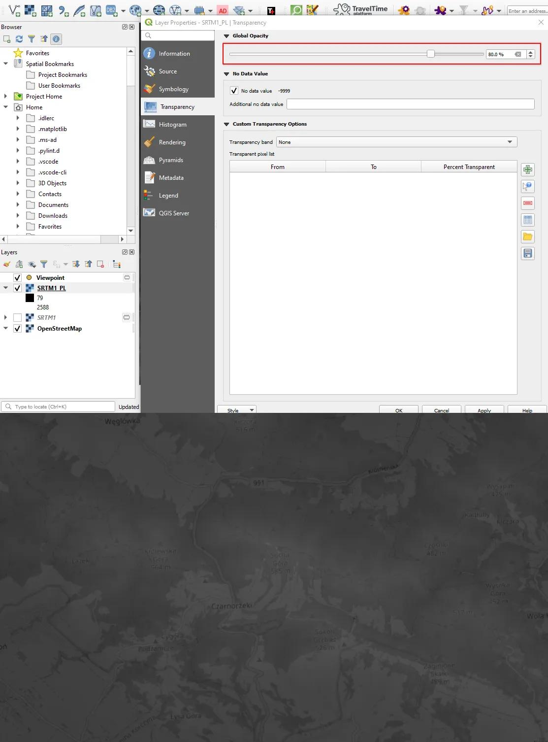
QGIS changing transparency of the raster layer

Pic. 11 Changing transparency of the raster layer and the results underneath. The reduction of opacity by just 20% gives a nice view of the OpenStreetMap canvas underneath.

Even a small reduction of the raster opacity can give you a satisfactory view of the map canvas underneath and help with locating your viewpoint.
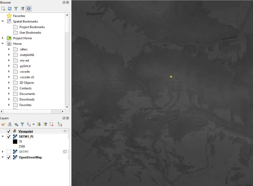
We can create one or more viewpoints. No attribute data are needed, they will be created by the Viewshed analysis plugin later on (Pic. 12).

QGIS create viewpoints for Viewshed analyses

Pic. 12 Creating viewpoint for Viewshed analyses in QGIS.

10. Once our viewpoint is created, we can use the Visibility analysis plugin.

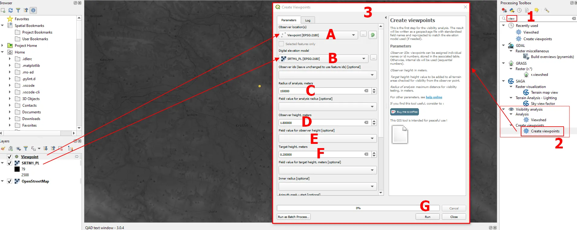
QGIS Visibiity analysis - create viewpoints

Pic. 13 Creating viewpoints in QGIS Visibility analysis plugin, where: 1 – Search phrase in Processing Toolbox; 2 – Selecting proper tool; 3 – The Create viewpoints panel; 3A – Loading Observer locations(s); 3B – Loading DEM file; 3C – Defining Radius of analysis (in meters); 3D – Defining Observer height (in meters); 3E – Providing Field value for observer height; 3F – Defining the Target height (in meters); 3G – Running algorithm.

The plugin tools can be found in the Processing Toolbox dockable panel. Use the search box there and start typing i.e. “view” or something like this (1). You should see the available options based on the selection. The Visibility analysis section will emerge at the bottom. Use the Create Viewpoints tool (2), which opens as a window with a few options (3). Now you should choose the Viewpoint layer, created earlier (3A), and the raster layer you are working on (3B). These layers are visible in the Layers panel and the red arrows show their place in the Create Viewpoints panel. Because of the matter of long distance observations the Radius of analysis will be quite large. Let’s assume it is 150km (150000 meters)(3C) whereas the Observer height should correspond to the standard height of an adult person (3D). The last one – the Target height (3F) is explained as the altitude above the ground level we intend to fly. It can represent the height of the object we might be interested in from an observer’s point of view. In the case of our study, this option will be explained later, as we need to see the results for the Earth’s surface first, but we can put some minimum values like 0.1 or 0.2 in order to create the attribute field just in case. It will allow us to play with these values in the future straight away without creating new viewpoints over and over again. In fact, by placing there i.e. 30m we would be able to visualize the potential visibility of the forested mountains from the given place. A case such as this will be analyzed later. We shouldn’t forget about other options available, which are marked as [optional] (3E). They apply both to the values provided straight away (3A-F) as well as a few others underneath, which will be considered later in this text.
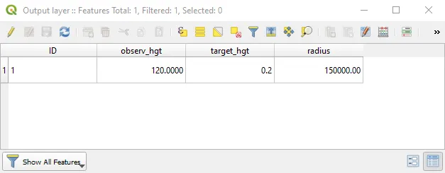
The result is our viewpoint equipped with the fields as defined beforehand (Pic. 14).

QGIS visibility analysis - New viewpoint created

Pic. 14 A New viewpoint was created with the fields defined beforehand.

III. MAKING VISIBILITY ANALYSES

Finally, we get to the point, where the data for visibility analysis is complete!

11. Use the Viewshed tool from the Processing Toolbox panel (Pic. 15).

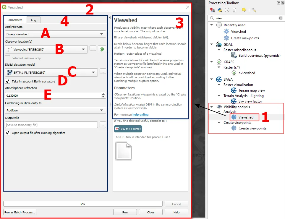
Viewshed tool in QGIS Visibility analysis

Pic. 15 The QGIS Visibility analysis – Viewshed tool options, where: 1 – The Viewshed tool in Planning Toolbox; 2 – The Viewshed window; 3 – The Viewshed instruction panel; 4 – The Viewshed options; 4A – Analysis type; 4B – Observer(s) location; 4C – DEM layer; 4D – Earth curvature on/off; 4E – Atmospheric refraction.

The same as the previous one, it can be found in Processing Toolbox panel (1) assuming, that you’ve typed the “view” phrase in the Processing Toolbox search bar. Double-click on it and the Viewshed window (2) will open straight away. Look at the instructions panel located on the right (3), which lists some basics in selections. Fill up all the inputs correctly (4) starting from the Analysis type (4A), which in our case should be Binary viewshed. This type of analysis throws the simplest results including areas, from the given point (or viewing platform) that are visible or not visible. As the Observer(s) location (4B) you should pick up the Viewpoint layer generated in the previous step. Look at the inactive option just below – Selected features only, which might help you to distinguish which exact viewpoints you want to include in your rendering, once have more than 1. The Digital elevation model file (4C) remains the same as usual because it’s the only raster file, we gained from merging and reprojection at the very beginning. A very important option, which unfortunately isn’t turned on initially is Take into account Earth’s curvature (4D). When missed, you might be surprised with your result, typical for flat Earth circumstances. The last bit to adjust is the Atmospheric refraction (4E). The default value of 0.13 corresponds to the standard terrestrial refraction coefficient. I am going to rediscuss this matter in the future, but for now, it can be left for testing purposes.
When everything is completed, please hit the “Run” button and wait a while for rendering. Depending on your PC or laptop parameters it might take a while, especially, that in the case of long-distance observations the values of radius are much higher than would be applied for typical archeological approaches as presented on the web.

The final result looks promising (Pic. 16). It’s been produced as another raster layer including just 2 colors – black (0 – not visible) and white (1 – visible).

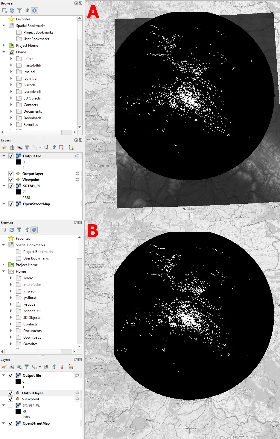
Pic. 16 The final result of viewshed analysis in QGIS. In the lower image, the DEM layer has been taken down from the map.

Now, the SRTM raster layer used across the whole process can be switched off as shown in the lower part of the image (Pic. 16).

IV. ALTERNATIVE APPROACH

As mentioned earlier, by the occasion of explaining the Viewpoint creation (Pic. 13), there are some empty inputs, which can be filled in just by providing the specified field and are marked as the [optional]. Essentially, we don’t need them for values such as Observer(s) height, Radius analysis, or Target height, as they are fillable in the Create Viewpoint window. However, there are others, that must be provided as the fields if we need some additional or alternative analyses (Pic. 17).

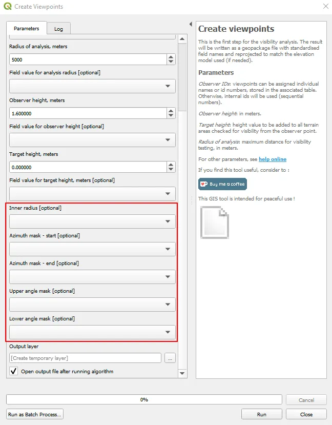
QGIS Visibility analysis - Create viewpoints additional elements

Pic. 17 Additional inputs, which are optional for the Viewpoint creation.

They are:
– Inner radius – defines another radius, in which the results will be excluded. By setting inner radius we can, for instance, set the range of distance in which the object visibility we are interested in. By excluding i.e. 50km from the observer point we will see the visibility cloak only beyond this distance.
– Azimuth mask – start & end – determines the range of azimuth we are interested in. It works on an analog basis, as typical (default) usage of Ulrich Deuschle panorama generator.
– Upper & lower angle mask – determines the maximum and minimum angle of vision and excludes the areas, which fall below or above these values. In fact, considering just long-distance observations these parameters won’t be particularly useful unlike browsing some archeological sites at much smaller distances from the viewing spot. For the purpose of extremely distant features, the vast majority of them will fall in the proximity of horizontal eye level at 0 degrees.
If you want to play with some of them, you must prepare the fields yet at the stage of scratch layer, created earlier in the QGIS project. Let’s go back to point 8, which explains the creation of a temporary scratch point layer.
This layer has been created without any fields, although in some QGIS versions, you can prepare them along with a selection of CRS and layer geometry.
If you haven’t done it, it’s not a problem, because the fields can be simply added to this layer later on (Pic. 18).
8B. Add the fields to the new temporary scratch layer only if you are planning to go with additional analyses available in the Visibility analysis plugin. Otherwise, there is no point in wasting your time, as the standard inputs can be done in the form as discussed earlier.

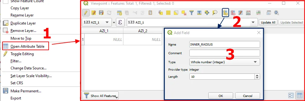
QGIS creating fields for scratch layer viewpoint

Pic. 18 Creating fields for the Viewpoint layer, which has been created earlier as the New Scratch layer.

You just need to right-click on the layer, you created earlier as the scratch one. Next, select the Open Attribute Table option (1). When opened use the Add field signature (2), which opens the Add Field window (3). Be mindful of the data type (Type) in the field you want to create. Because we need the azimuth and radius they should come as a Whole number (integer). We don’t need decimals here, nor do strings. Remember, that the inner radius value should be expressed in meters. Therefore you should adjust the proper value Length, which safely should count to 10, whereas 3 for azimuth should be fair enough.

9B. Once fields are created, you can provide your own data adequate to the viewpoint circumstances and your own expectations.
Let’s assume, that our first azimuth is 110, the second one 180, and the inner radius will count 25km (25000 meters). Cutting down the azimuth range (which in default is 360° exactly) should reduce the waiting time for viewshed rendering. The same applies to applying the inner radius or reducing the main radius. This information is important for users, who don’t own good laptops.

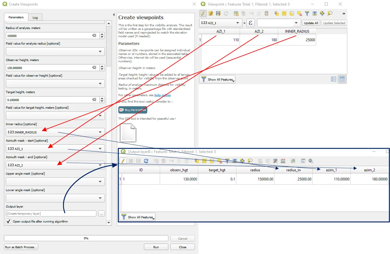
QGIS Visibility analysis - Viewpoint creator - additional options

Pic. 19 Additional options for viewpoint creation. After preparing the attribute table, the fields can be included in the Create Viewpoints options. When the output file is rendered, it includes them in the attribute table.

The attribute table of the Output layer is crucial, as it’s used by the Viewshed tool for rendering the visibility cloak.

10B. The final result will be different than the standard one (Pic. 20).

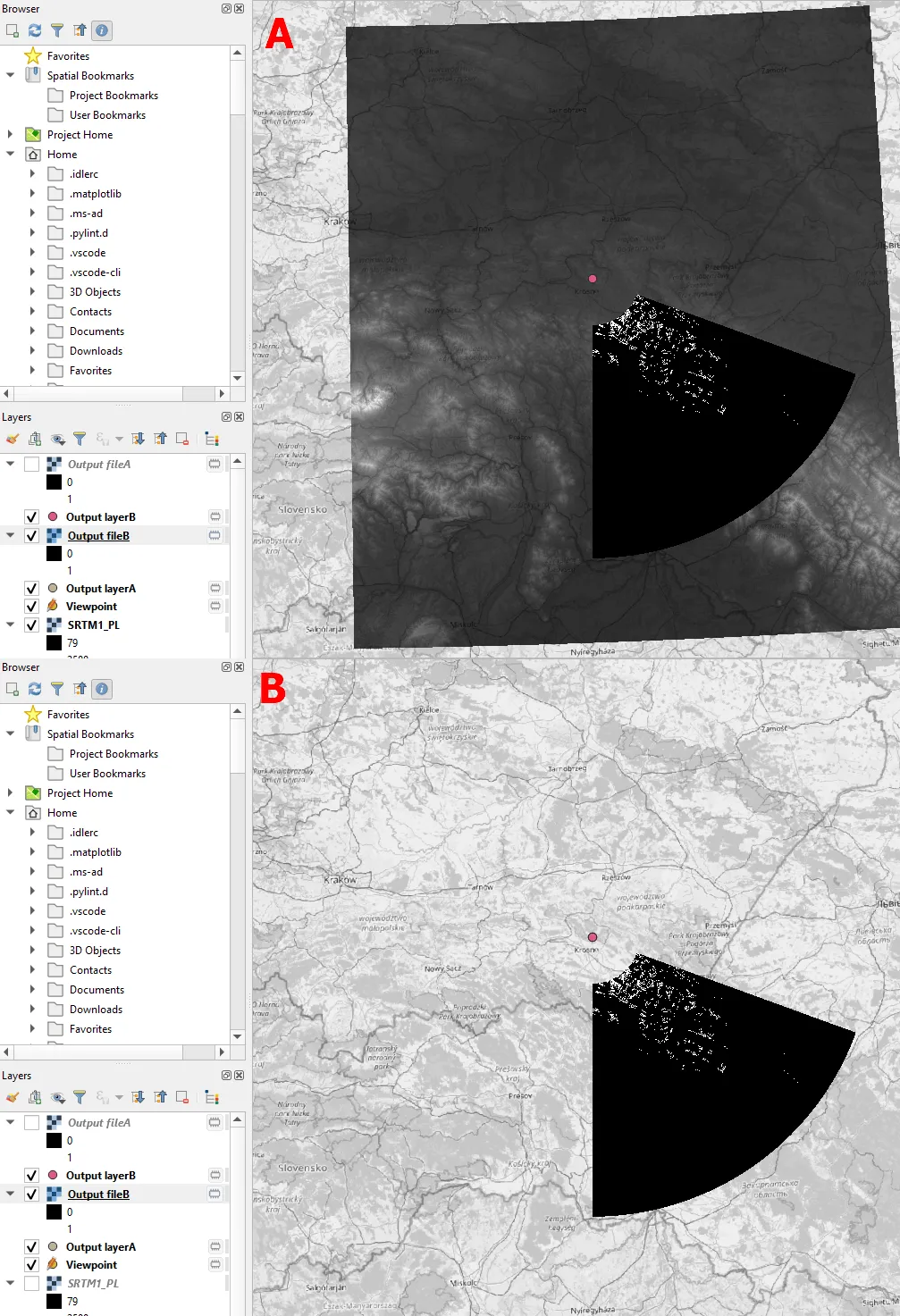
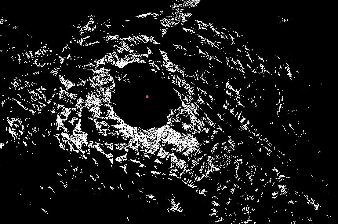
Pic. 20 The final result of additional visibility analysis, which includes the minimum distance (inner radius) and azimuth range. The same as previously, the comparison with and without the DEM raster in the background.

When applying the angle range instead of azimuth and inner radius, then the result will be also interesting. For the angle range between -2 and 0 degrees, we can clearly see, that objects located close to the elevated viewpoint are simply not included. Because our place has an elevation of about 710m.a.s.l (the altitude of the peak + elevation range) compared to surrounding hills counting at most 530m.a.s.l. the closest of them are visible under a much lower angle than considered (Pic. 21).

QGIS Viewshed analysis final version angle range

Pic. 21 The final rendering of the visibility cloak when the angle range between -2 and 0 degrees has been taken into account. We can clearly see, that the grounds located closely to our elevated viewpoint aren’t considered in this analysis.

V. VISIBILITY CLOAK VISUALIZATION

When our Output files with visibility cloak are done, we are still rather unable to read them properly. This is because the output raster layer comes in full opacity.

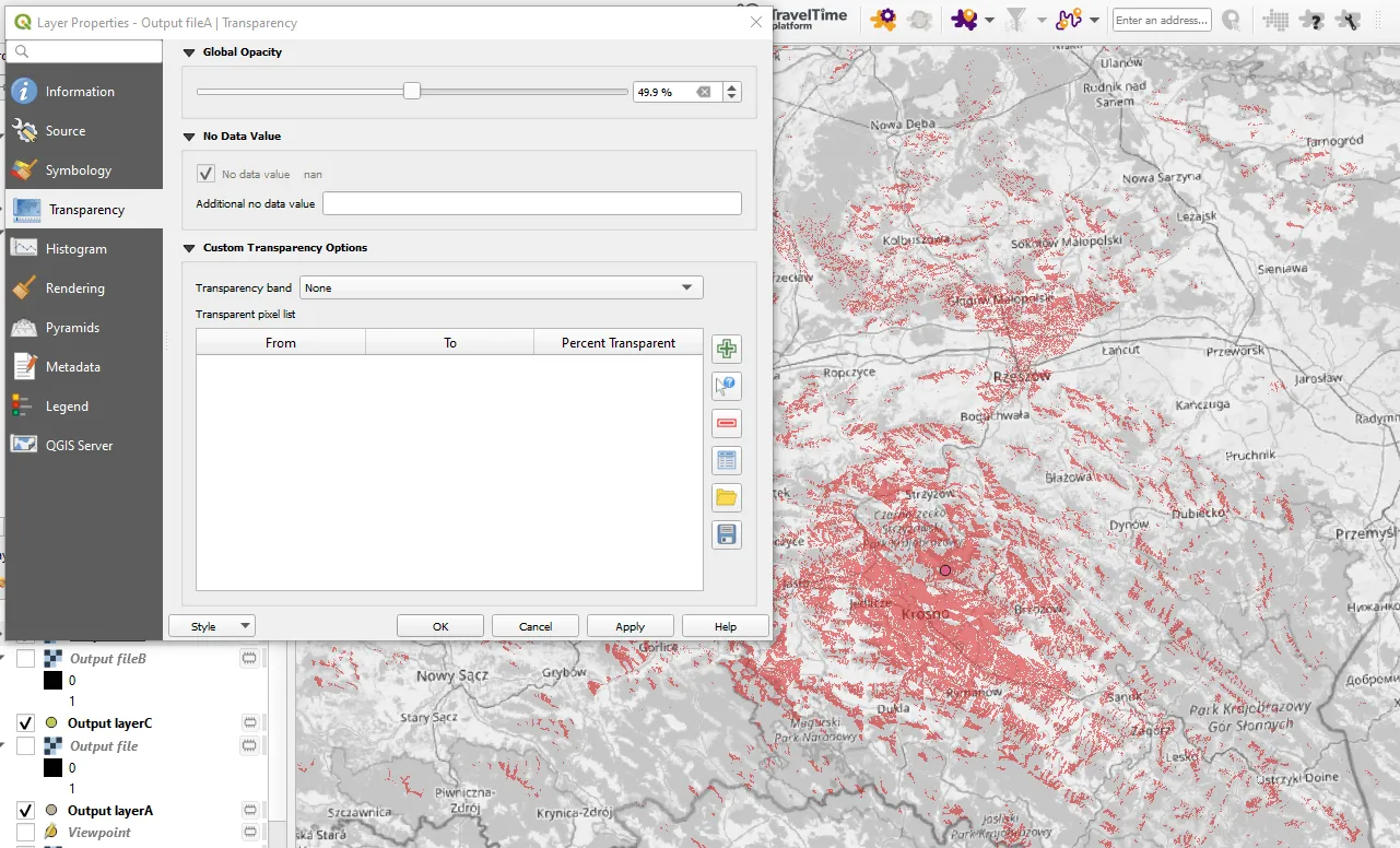
12. The first attempt for visualization of our output visibility cloak is changing the transparency of our raster. This is the most basic and fastest thing we can do in order to get around quickly with our results. Find your output layer in the Layers panel -> double-click -> Properties -> Transparency and reduce Global Opacity from its default value of 100% to the lower amount, by which you will be able to identify the map tile features underneath (Pic. 22).

QGIS visibility cloak changes of opacity

Pic. 22 Changes of opacity level in our visibility cloak raster produced by the Viewshed tool. The default opacity value is 100%, but reduced by half gives a chance to see the map underneath quite clearly.

13. Show only visible areas by changing the symbology of your raster layer.

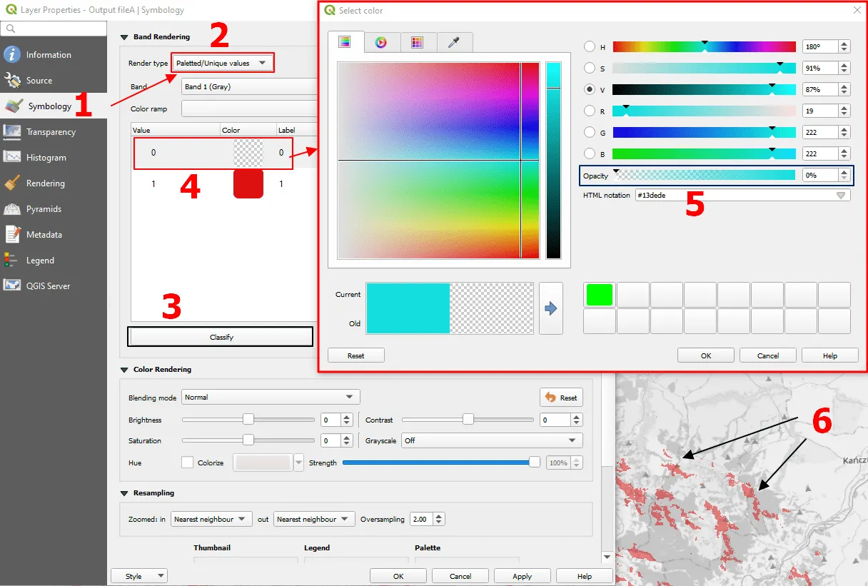
Pic. 23 Adjusting the visibility cloak raster layer style, where: 1 – The Symbology option; 2 – Selecting Raster rendering type as Palette/Unique values; 3 – Classification unique values; 4 – Classified band values for the produced visibility cloak; 5 – Removing (decreasing to 0%) opacity for one of them.

When your visibility cloak raster layer is completed, right-click on it and navigate to Symbology (1) where you should focus on the Band Rendering section. Your default render type is surely the Singleband gray. Please change it to Palette/Unique values (2). In fact, alternatively, you could use the Singleband pseudocolor option, but it’s used rather for rasters with multiple bands. We have just 2. Since the total number of your bands is low (2 or at most several) you can stay by Palette/Unique values. By clicking the “Classify” button (3) at the bottom, you will receive the total number of bands detected by the tool. As a result of the viewshed analysis, only 2 bands should have appeared (0 – not visible and 1 – visible). Important is to make a visual switch off the one, that corresponds to Not visible areas. This is simple by double-clicking on the color box and decreasing the opacity totally (5). The opacity of another box, which matches visible areas should have an opacity of 100%. Remember, that this is only local opacity. It means, that its value of it is reliant on the Global opacity discussed earlier (Pic. 22, 24). So even if it’s set to 100% it will represent 100% of the Global opacity amount. Let’s imagine, that your Global opacity is set at 50% as discussed earlier. When the local opacity of this particular band is 100%, then its visible opacity will be 50% (Pic. 24). Once local opacity decreases to 80%, and the global one is kept at 50%, the visible one will be just 40%, and so on

Pic. 24 The raster layer with our visibility cloak with adjusted style and global opacity set to about 50% value.

This is still just a raster layer. Sometimes we would need more sophisticated analyses, which can be done only with vector layers. For this purpose, the appropriate transformation is required.

14. Vectorize your raster output. You can do it easily by navigating to the top Main Bar -> Raster -> Conversion -> Polygonize… (Raster to Vector).

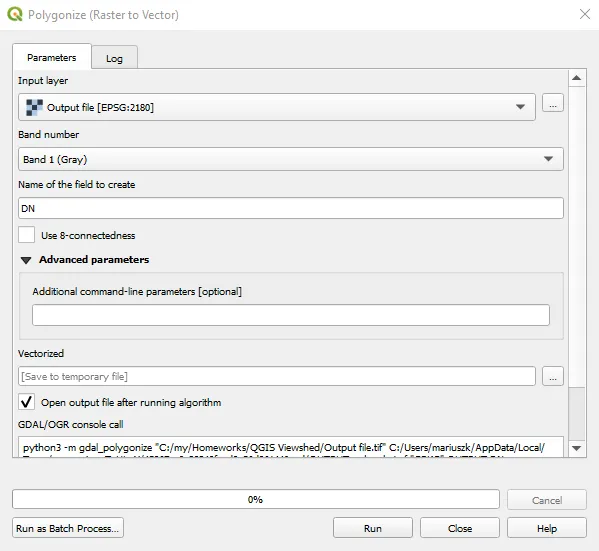
Pic. 24 The Polygonize (Raster to Vector) window with options selected.

Next, the following window will pop up (Pic. 24), which includes a few options. You just need to provide the Input layer and leave the other ones as they are. Optionally you can change the Name of the field to create, which will appear in the attribute table later.
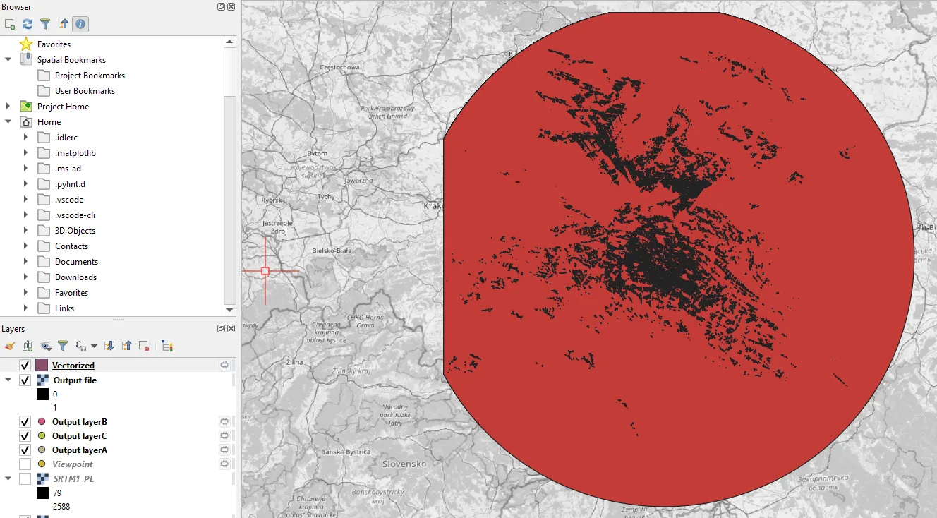
Execution of the algorithm might last quite a long when your PC is not strong enough. When done, you should see the Vectorized output file with details retrieved accurately (Pic. 25) and overlapping the raster Output file ideally.

Pic. 25 Vectorized visibility cloak in QGIS, which overlaps the raster Output file ideally with all details retrieved accurately.

Unfortunately, we still cannot work with this data. They must be extracted.

15. Extracting the visible areas can be done by selecting them in the attribute table. A bit earlier I mentioned the Name of the field to create option, which defines the name of the newly created field including the band value known from the raster Output file.

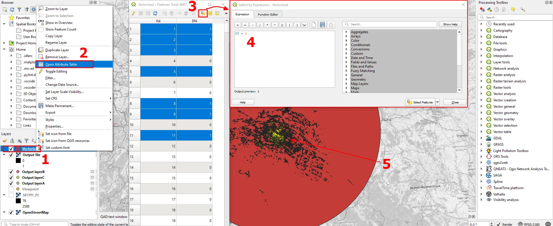
QGIS vectorized visibility cloak - select visible areas

Pic. 26 Selecting visible areas from the vectorized visibility cloak raster output file, where: 1 – Right-clicking on the Vectorized layer; 2 – Selecting Open Attribute Table option; 3 – Selecting “Select by Expression” tool; 4 – The selection formula; 5 – Selected content within the Vectorized layer.

Now, after right-clicking on your Vectorized layer (1), select the Open Attribute Table (2) option. When opened, you should see two fields. One of them is fid (the ID number) and another one is generated by the Polygonizing algorithm discussed earlier. Because we haven’t changed the name of this field (Pic. 13) it’s exactly the same here. It represents numbers adequate for the band values comprising our raster Output file (Pic. 16). We need just the number 1, which corresponds to the Visible areas from our viewpoint. For this purpose, you need to use the “Select by the expression” tool (3) and provide the following formula (4):

DN = 1
or
your_field_name = 1

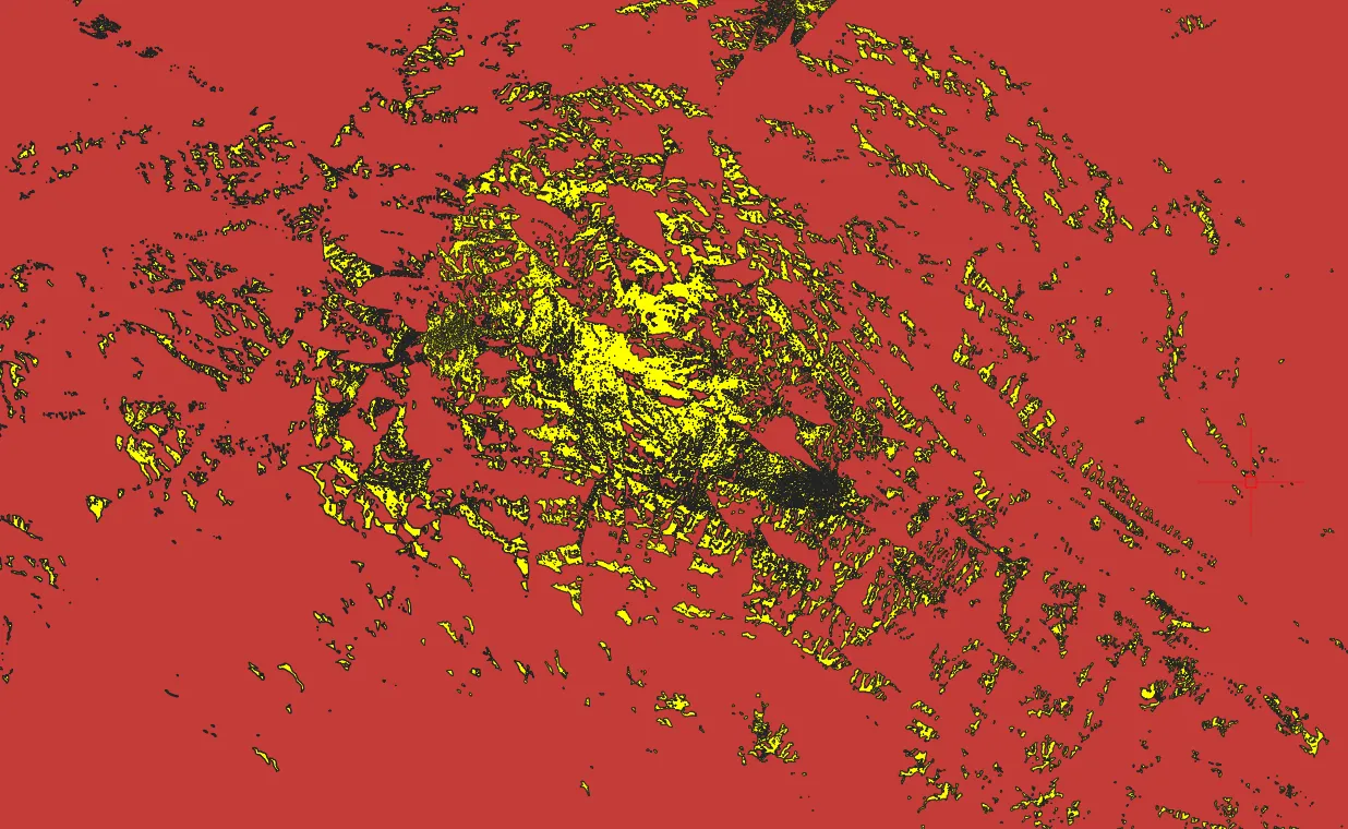
, and click the “Select Features” button in the bottom right corner. The result is visible after a while, depending on the strength of your computer. All the selected elements have changed their color to yellow (5) (the default selection color in QGIS, which can be always changed) (Pic. 27).

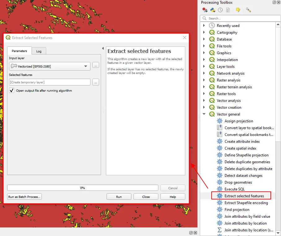
QGIS Viewshed vector layer selected visible areas

Pic. 27 Selected space, which represents the visible areas from our viewpoint.

Since the proper data is selected, there are two ways of extracting it. The first one is to be found in the Processing Toolbox -> Vector General -> Extract Selected Features (Pic. 28).

QGIS Processing toolbox Extract selected features

Pic. 28 The Extract Selected Features tool and its location in the QGIS Processing Toolbox.

The second one it’s more traditional and can be accessed by right-clicking on our Vectorized layer.

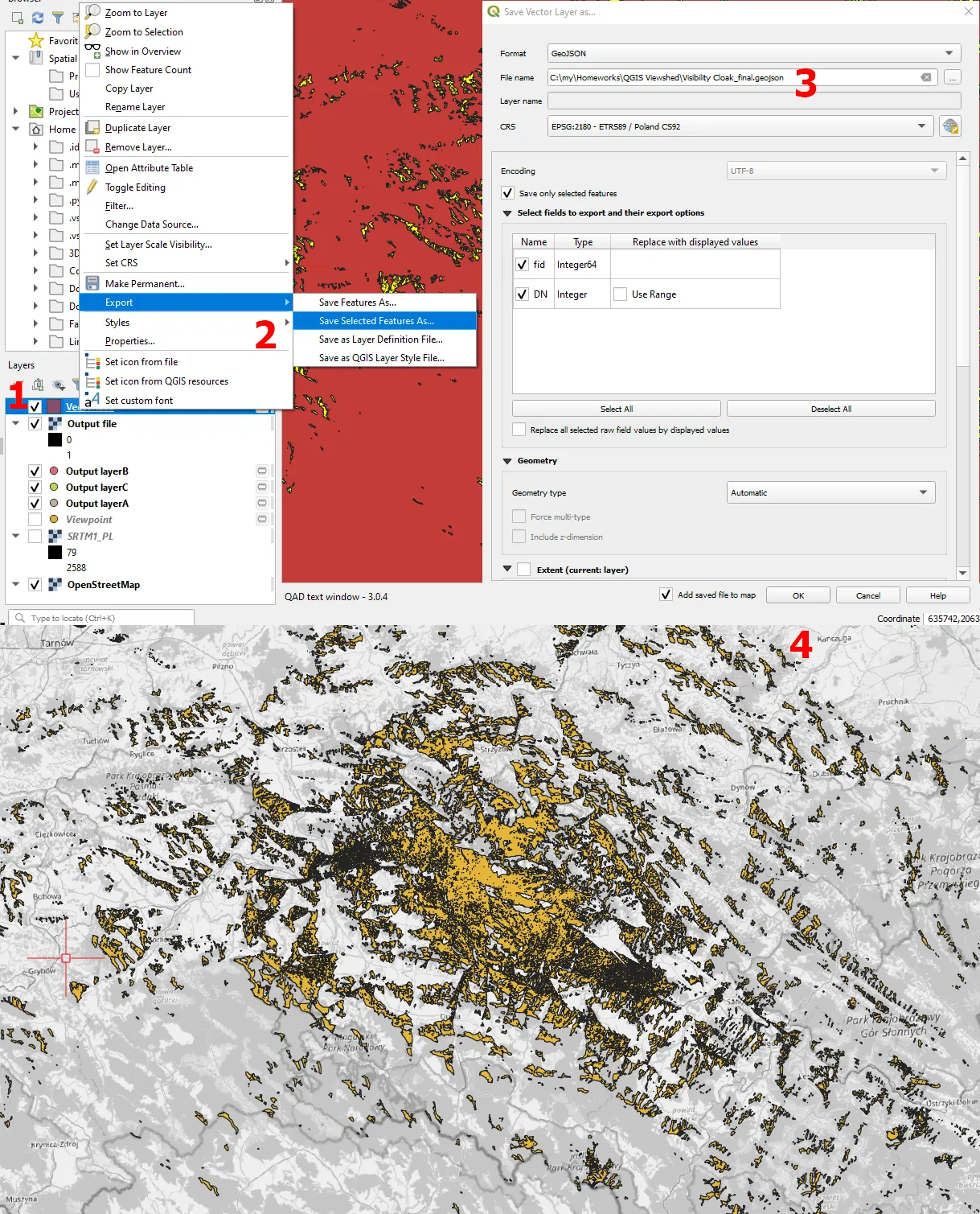
QGIS Visibility cloak export selected features

Pic. 29 The traditional “Export selected features” option in QGIS, where: 1 – Right-clicking on the layer; 2 – Selecting Export -> Export Selected Features As… option; 3 – Providing filename & path directory; 4 – Extracted visible areas.

After right-clicking (1) select Export -> Save Selected Features As… (2), next provide the filename and its target directory (3) and click OK. Finally, after turning off all other layers, you should see only the extracted vector bits, which correspond to the final visibility cloak rendered from the Viewpoint defined at the very beginning of our work. In fact, the view isn’t neat enough, therefore the last small step might be optionally required.

16. Styling extracted visibility cloak vector layer is an easy fix, and plays just around the stroke of the shapes (Pic. 30)

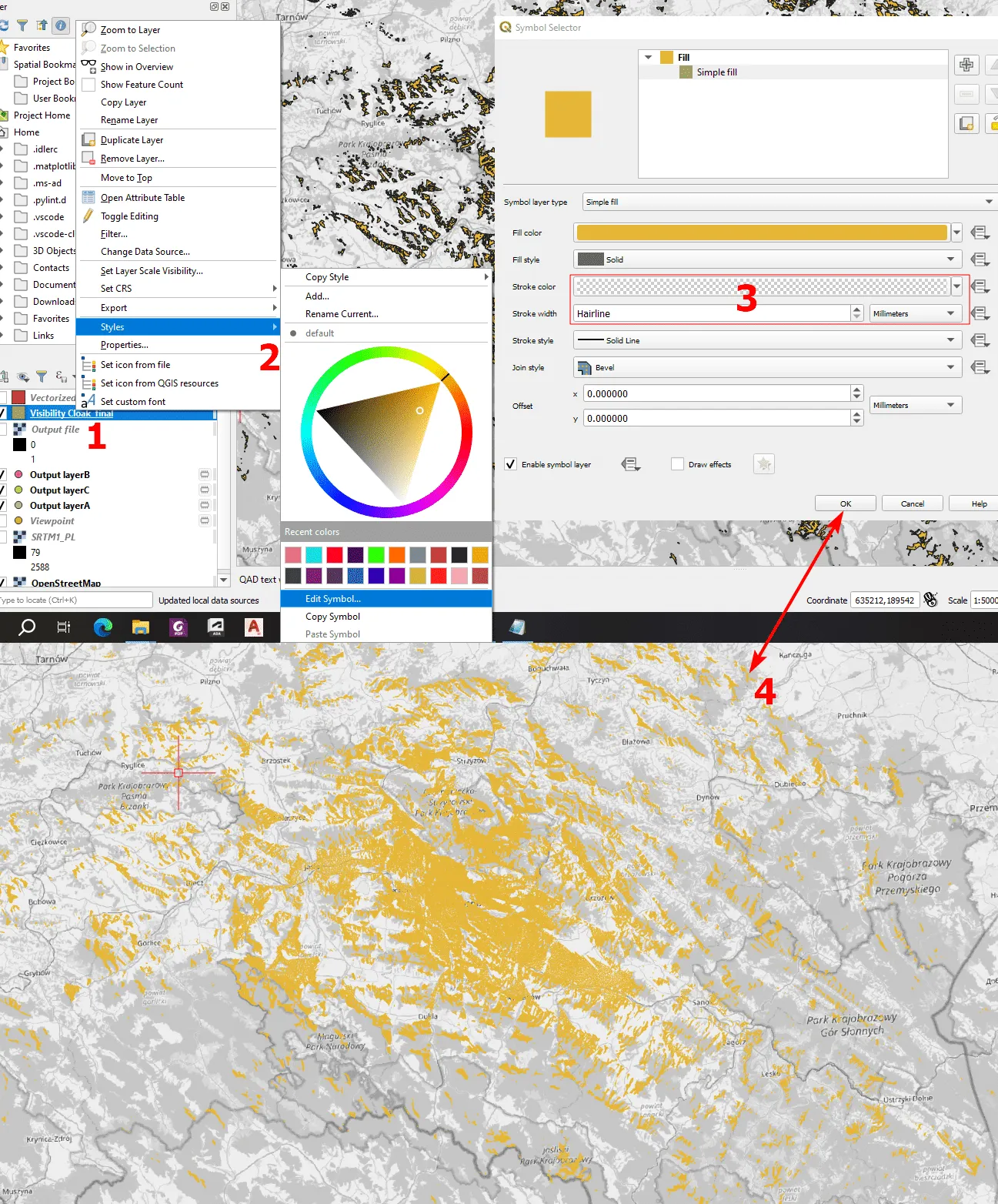
QGIS Visibility cloak styling vector layer

Pic. 30 Styling the final visibility cloak vector layer, where: 1 – Right-clicking on the layer; 2 – Selecting Styles -> Edit Symbol; 3 – Setting Stroke color as full transparent with the Stroke width of 0 (Hairline); 4 – Clicking OK and applying changes.

By right-clicking on our extracted visibility cloak layer (1) navigate to Styles -> Edit symbol (2) and set 2 stroke parameters like shown in the image above (Pic. 30, 3). Optionally you can change the color either here. After hitting the “OK” button, we should see the changes quite quickly (4). Now, our visibility cloak looks almost the same as discussed earlier (Pic. 23) and as known from the Heywhatsthat.com service. The matter of the visibility cloak gained from Heywhatsthat.com has been discussed a while ago by myself, but I will back to it with another solution soon. I am going also to carry on the usage of the visibility cloak with various vector QGIS analyses, which will constitute the continuation of this particular part of the thread.

VI. OTHER ANALYSES

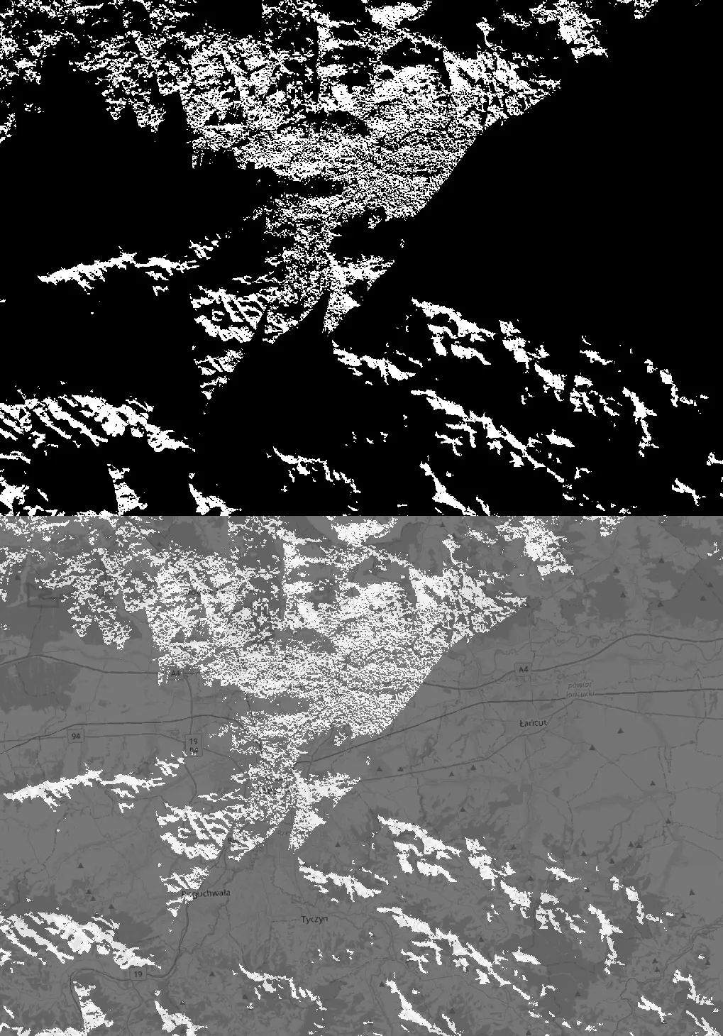
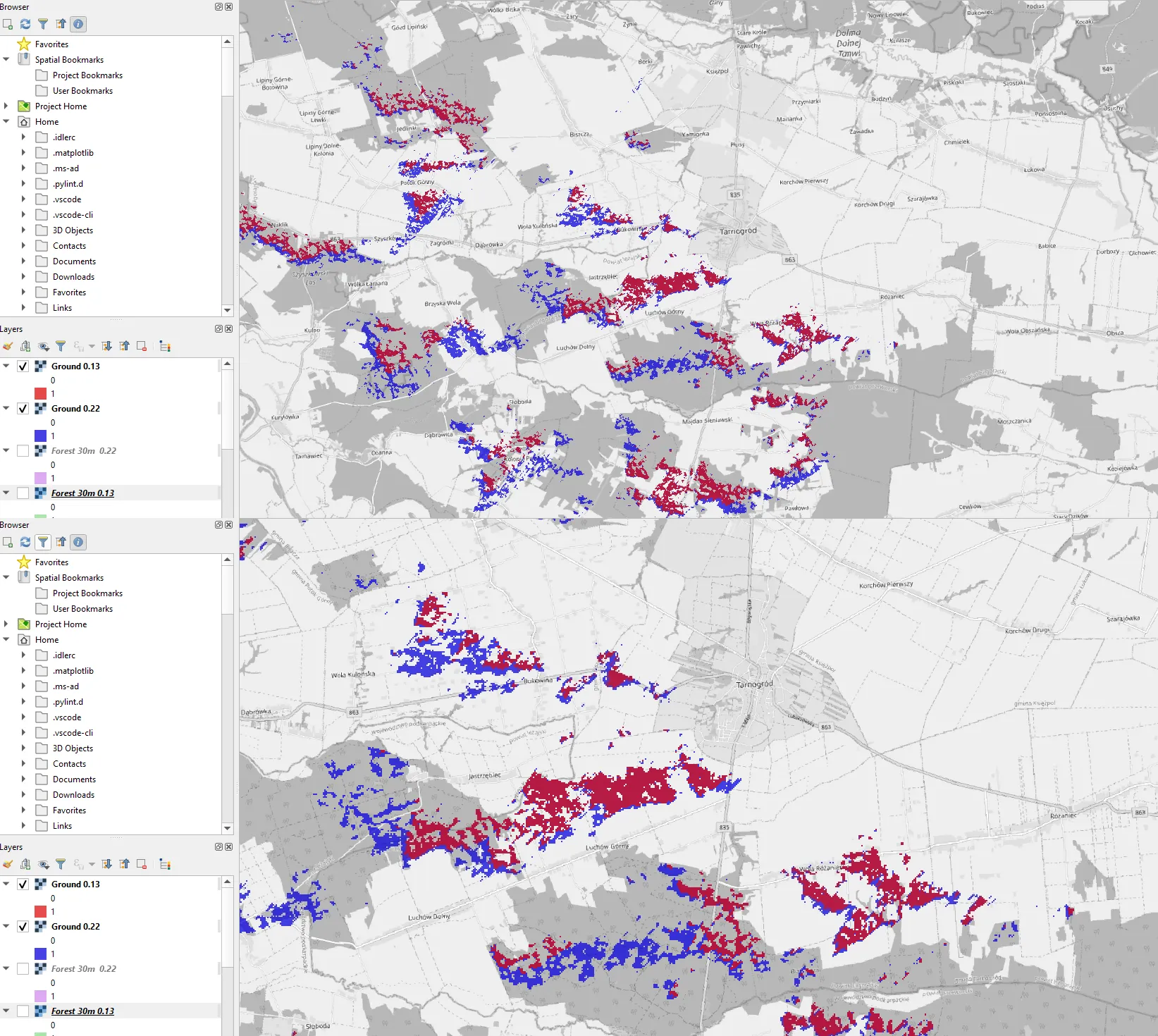
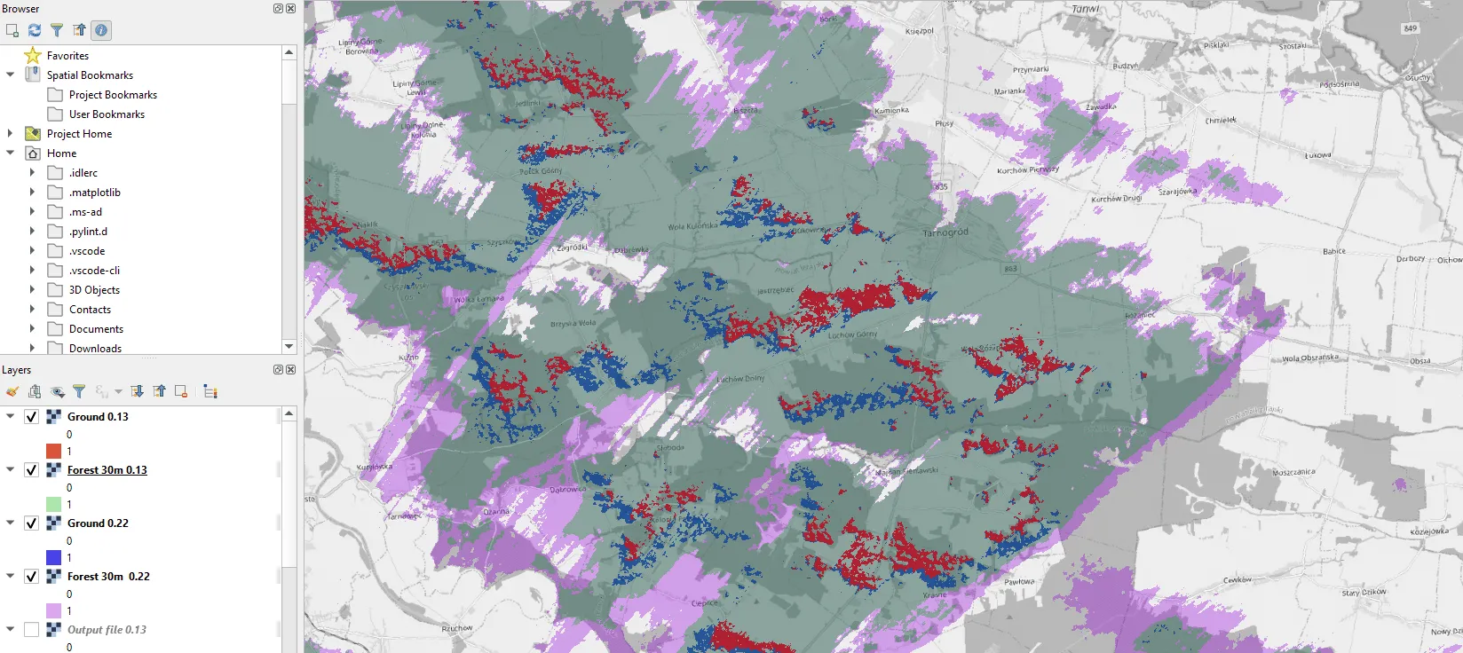
It has been told before about two other crucial options, which would play an important role in making proper viewshed analyses with respect to the various circumstances. These elements are the atmospheric refraction and the target object altitude. The first element is default set in a standard value of 0.13, but sometimes the abnormality can lift this coefficient up to 0.22 locally. This particular matter will be also discussed in the future, but for the time being, I just prepared two situations in which you can see the difference in visibility cloak rendered by the Viewshed tool (Pic. 31).

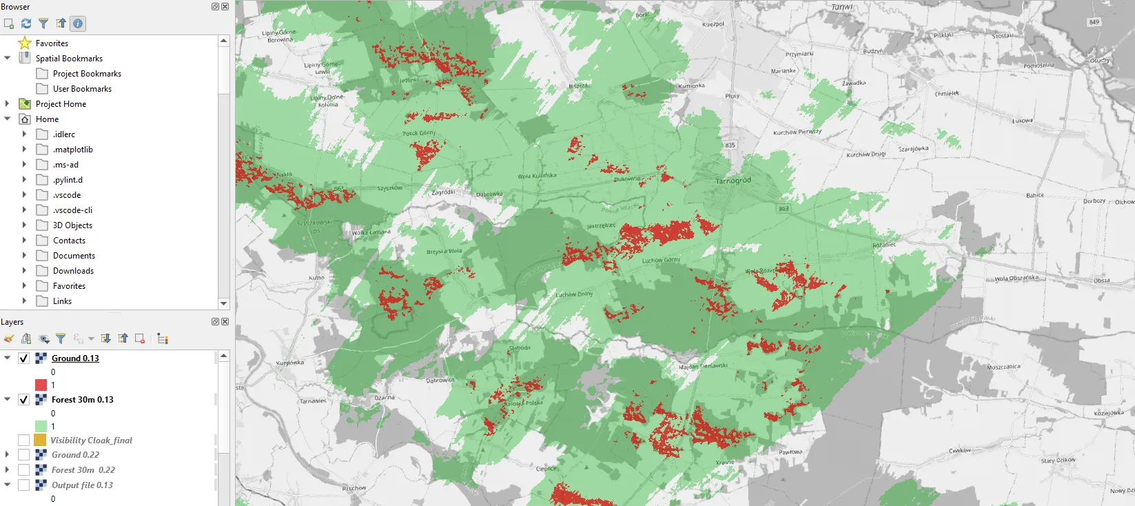
$QGIS Visibility cloak rendering for various refraction coefficiient$

Pic. 31 The visibility cloak rendered for various refraction coefficients, where: Red – standard 0.13; Blue – abnormal 0.22 as per the styling visible in the Layers panel. Click to enlarge.

A much bigger difference with the visibility cloak will be seen once the different heights of the target object are applied. The image above (Pic. 31) represents the classic situation, as known from all of the tools dealing with Visibility analyses. Namely, the only foundation of the viewshed computations is DEM, which in other words is just the pure ground. If you use, for example, Heywhatsthat.com, you will get the visibility cloak for the given viewpoint, in which the target object height will be 0m in every direction, as the ground level is considered.
By increasing the target height, our area of visibility will effectively grow. Imagine, that the standard forest height is about 30m, so let’s set our Target height at 30m then. Now, the visibility cloak will show all areas visible at a height of 30m exactly. By way of explanation, we are computing all the potential places, from which our viewpoint is visible from this altitude. So for extremal ranges, it will play an important role, because of showing the areas, from which our viewpoint wouldn’t be visible without applying this 30m altitude (Pic. 32).

QGIS visibility cloak with the treeline height.

Pic. 32 The comparison of the visibility cloak for the ground conditions and with the standard treeline height applied. Click to enlarge.

As you can see, the 30m of standard treeline height changes the visibility cloak significantly! Of course, the abnormal refraction coefficient will increase the visual range a bit more (Pic. 33).

$QGIS visibility cloak including refraction and treeline height of 30m above ground$

Pic. 33 The visibility cloak generated in QGIS, which includes all 4 situations considered in this article: Red – ground with a standard refraction coefficient of 0.13; Green – forest height of 30m with a standard refraction coefficient of 0.13; Blue – ground with abnormal refraction coefficient of 0.22; Purple – a forest with abnormal refraction coefficient 0.22. Click to enlarge.

The target altitude can be needed for estimating the potential line of sight between two artificial objects. It’s the parallel method to the one described here, which takes into account the limits of visibility cloaks rendered from Heywhatsthat.com. Here, by setting the target altitude i.e. 50m, we can gauge the potential line of sight between our viewpoint (which can be elevated anytime) and some other man-made object like a tower, transmitter, high-rise building, HV electric pole, and so forth. By converting the generated visibility cloak to the vector layer shown earlier (Pic. 29), analyses such as this could be done in a bunch for several objects. I guess, firstly the coverage of these objects for the analyzed area would be needed, but it’s a matter for further deals.

VII. SUMMARY

The correct usage of the QGIS Viewshed analysis plugin can result in the creation of valuable viewshed maps from each observation point. Subsequently, likewise in the case of rendering viewsheds for a whole ancient town, the same can be applied to the viewshed of a whole mountain range. The other appliance of this plugin can be Intervisibility describing all intermediate points residing along the line of sight between our viewpoint and the most distant object observed. Another curious feature of the Visibility analysis plugin can be the visibility index of 2 or more objects. In a graphical sense, the user receives a colored map, which can read from where 1, 2, or more objects are visible at once, something similar to this obsolete method. Moreover, I was focused on explaining the viewshed analysis just for one particular viewpoint. Of course, with the Visibility analysis plugin, you can do the computations for a multitude of them. There are no restrictions on the total number of viewpoints, hence we can guess that the upper limit is marked by the capacity of your computer. Contrary to the single viewpoint simulated usually for some mountainous or elevated areas, there is an option for the creation of a chain of viewpoints located close to each other, which would produce the estimated visibility cloak even from the whole road section. We must know, that before reaching some interesting place we travel some distance and make interaction with the regional landscape (Quinn, 2022).

It’s vital to list all the pros and cons of this method by comparing it to i.e. the Heywhatsthat.com service, which serves as an analog visibility cloak product for the given viewpoint.

PROS:

Many options for characterizing the user’s viewpoint – there is no other tool, that would offer more than this plugin,
The Create Viewpoint tool can be used just once – because the user can adjust the attribute field values manually later,
The visibility cloak can be rendered with including the refraction coefficient – this is a very convenient option rather unavailable elsewhere,
The option for setting the target height of the observed object – allows you to answer the question, could I be visible from that object?
The possibility of reducing the azimuth range, angle range, and inner radius – which should help you to get the desired result much quicker,
A quick way of visualization at least for raster output – without hassle, you can simply classify the bands and adjust their colorations & opacities
The plugin is under development – unlike other parallel tools, this item is growing up and it’s highly likely, that will be equipped with other interesting options in the future

CONS:

Time-consuming preparation of the DEM files – even if you use other services, than presented in the example, the workaround might take some time, unlike for example Heywhatsthat.com, where the simulations can be obtained much quicker.
Visibility cloak restricted to the area of analysis – despite the much larger visibility cloak, that could be obtained (sometimes) from the given viewpoint, the user receives only the bits restricted by the DEM file provided.
Clumsy processing driven by large datasets – is not always compatible with the strength of your computer
The raster layer is a default output file – which requires an essential transformation to the vector one if various analyses are needed

All the advantages and disadvantages presented above compare the QGIS Visibility analysis plugin to other parallel applications especially Heywhatsthat.com, which gives the same graphical pattern for the visibility cloak output. For the final conclusion, the plugin is definitely worth using and I hope, that my background, quite often omitted in other sources will help you produce successful viewshed maps.

Mariusz Krukar

References:

Achilleos G., Tsouchlaraki A., 2004, Visibility and viewshed algorithms in an information system for environmental management, (in:) WIT Transactions on Information and Communication Technologies
Bruy A., Svidzinska D., 2015, QGIS by example, PACKT Publishing, Birmingham – Mumbai
Čučković Z., 2016, Advanced viewshed analysis: a Quantum GIS plug-in for the analysis of visual landscapes, (in:) The Journal of Open Source Software 4(1)
Fisher P. F., 1996, Extending the Applicability of Viewsheds in
Landscape Planning, The American Society for Photogrammetry and Remote Sensing
Lockwood E., Masters P., 2021, Application of viewshed analysis and probability mapping for search area determination based on the Moors murders on Saddleworth Moor, the United Kingdom, (in:) Journal of Forensic Sciences 66(5):1770-1787
Mineli A., et al., 2014, An Open Source GIS Tool to Quantify the Visual Impact of Wind Turbines and Photovoltaic Panels, (in:) Environmental Impact Assessment Review 49:70 – 78
Mostafa M., 2023, Investigation of the most suitable observation points in natural resources monitoring using spatial analysis, (in:) Journal of Geography and Environmental Hazards, Vol. 12, i.1, SN 45
Quinn S.D., 2022, What can we see from the road? Applications of a cumulative viewshed analysis on a US state highway network, (in:) Geographica Helvetica 77, p. 165-178
Ren L., Cao Y., 2021, GIS-based viewshed analysis on the conservation planning of historic towns: The case study of Xinchang, Shanghai, (in:) The International Archives of the Photogrammetry, Remote Sensing and Spatial Information Sciences, Volume XLVI-M-1-2021
Saxena V., Mundra P., Jigyasu D., 2020, Efficient viewshed analysis as QGIS plugin, (in:) 2020 2nd International Conference on Advances in Computing, Communication Control and Networking (ICACCCN)